Data driven literary analysis

Why am I doing this?

When I was in high school my studies were heavily skewed towards foreign languages and literature in general. This means that between ages 14 and 18 I wrote a whole lot of literary analysis essays. The idea behind this exercise is that if you analyze and describe the techniques that make a piece of literature effective, you’re more likely to understand how and why that piece has been written.

Some 10 years later I became interested in Natural Language Processing (NLP). What I found most fascinating is the idea of machines understanding human languages, a task that humans often fail at. As a result, I spent most of my time at the Recurse Center teaching myself about NLP and playing with Shakespeare’s body of work in the attempt to automate the process of writing a literary analysis essay.

This article is a summary of what I learned and the method I came up with.

What is natural language processing?

Natural Language Processing is a field of computer science studying all interactions between natural and artificial languages. Natural languages are those used in every day communications between humans, and are the result of constant evolution through time and usage. Artificial languages are constructed for a specific purpose (think mathematical symbols or programming languages).

In a broad sense, NLP includes all computer manipulations of human languages, from simple word counts to understanding human utterances. By enabling computers to understand as well as generate natural, human language, they can be used for a wide range of everyday applications, like machine translation and spam filtering.

Some of these methods can easily be applied to literary texts to extract structure and meaning.

Genre classification

The first step in the analysis of a piece of literature is identifying what category it belongs to. This task is essentialy Document Classification, the process of assigning one or more labels to a document. This is generally a supervised problem, where labels are predifined and assigned to the input documents prior to training the model.

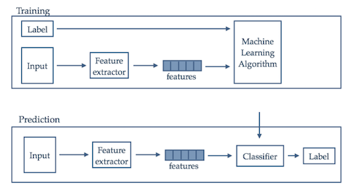
The issue with this approach is that it requires a large collection of labelled documents to train the prediction model. When a labeled set is not available someone has to manually tag the documents in the corpus prior to the training stage. This can be time consuming.

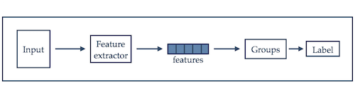
The alternative is an unsupervised approach. Groups are created with the goal of capturing, or extracting, the natural structure in the data. When this is done correctly it is possible to inspect only a subset of each group and attach a label to each of them.

Shakespeare analysis: classifying plays

Shakespeare is best known for his plays, most of which were produced between the end of the 16^th century and the beginning of the 17^th century. There is some controversy regarding whether all the plays were written by the same author, but scholars generally agree on dividing them into three categories: comedies, tragedies, and histories. I’m going to leave the histories out of the analysis because they’re much harder to define, and focus on the differences between the other two categories, comedies and tragedies.

Comedies tend to focus on situations rather than characters. Multiple plot lines that see characters separated and reunited, use of puns, identity confusion, family conflicts, and young love are all common traits of Shakespeare’s comedies.

Tragedies focus on characters over plot and emphasize their honesty or lack thereof. The plot is generally more linear and follows a classic definition of tragedy in which a hero of noble birth is brought to ruin by some tragic flaw.

Shakespeare wrote 17 comedies and 10 tragedies for a total of 27 plays and a vocabulary (excluding stop words¹) of over 11,000 words (the features). This influences the analysis in two ways:

• The number of features: in high dimensional spaces, all objects appear sparse and dissimilar, which makes it really hard to efficiently organize them in groups based on similarities. I use content-based feature extraction to represent the document in a lower number of dimensions.
• The size of the training set: the number of documents is simply too small for a model to learn the differences between classes. Instead of learning pre-defined categories I use a clustering algorithm to find the best two-way split of the set and compare it to the traditional classification.

Step 1: Content-based feature extraction

Feature extraction is a general term for methods that convert raw data into a set of derived values, called features, intended to be non-redundant and informative. When the initial set of inputs is too large or redundant, feature extraction facilitates learning by feeding the classification algorithm with a reduced representation of the data containing the information relevant to the task, rather than the initial complete set. This is very domain specific and depends on the available data.

In the example, it’s important to extract the semantic information in the text so that it can easily be interpreted by a machine. A simple way of doing this is using tf-idf, a statistical score for the importance of words in both the document and the corpus. Tf-idf, however, doesn’t reduce the number of features. For that, we’ll use topic modeling. Topic modeling allows us to extract features that describe the content of the corresponding document, representing it in the form of word distributions, revealing hidden semantic structures in the text.

Latent Dirichlet Allocation

Latent Dirichlet Allocation is a topic modeling technique that describes the probabilistic procedure used to assign words to documents.

In this context:

• a word w is an item from a vocabulary indexed $\{1, ..., V\}$
• a document is a sequence of N words denoted by $\mathbf{w} = (w_1, ..., w_N)$ where $w_n$ is the nth word in the sequence.
• a corpus is a collection of M documents denoted by $D = \{\mathbf{w}_1, .., \mathbf{w}_M\}$

Given a collection of documents, and K topics, LDA finds the formal relationship between the observed frequencies of the words in the documents and the latent topics, where a topic is characterized by a distribution over words. For example, assume our vocabulary is made up of the words panda, broccoli, cat, eat and apple. A topic about cute animals will assign higher probabilities to panda and cat (e.g. P(panda) = 0.3, P(cat) = 0.3, P(eat) = 0.15, P(apple) = 0.125, P(broccoli) = 0.125), whereas a topic about food would assign them lower probabilities (e.g. P(panda) = 0.05, P(cat) = 0.05, P(eat) = 0.3, P(apple) = 0.3, P(broccoli) = 0.3).

The process that describes documents generation has 3 steps.

For each document:

1. Select the number of words
2. Draw a distribution of topics $\theta ~ Dir(\alpha)$
3. For each word $w_n$ in the document:
   • Draw a specific topic $z_n ~ Multinomial(\theta)$
   • Choose a word $w_n$ from $p(w_n \vert z_n, \beta)$, a multinomial probability conditioned on the topic $z_n$

What is most interesting about LDA is the use of the Dirichlet distribution, which is particularly useful for modeling the randomness of probability mass functions (pmf). A pmf gives the probability of a discrete random variable to take a specific value. A simple example is a 6-sided die, where in order to select a random value we roll the die and produce a number from 1 to 6. In theory, each number has the same probability of being selected, but in real life, due to the laws of physics and manufacturing, each die is slightly different and represents a different pmf. If we have a bag full of dice and we randomly extract one of them we are effectively drawing from a random pmf. This can be modeled with a Dirichlet of parameter $\alpha$.

In the context of text analysis, a document is a pmf of length V (the number of words in the dictionary) and a collection of documents produces a collection of pmfs. In LDA topics are latent multinomials so we can use the Dirichlet distribution to describe the probability of each topic in each document. Ultimately, this means that LDA can be used to extract topics in form of words distributions and then represent each document as a mixture of topics².

Running LDA on the collection of plays attributed to Shakespeare, we obtain the probability distribution of the words in the dictionary for each topic. By looking at the words that have highest probability in the topic it is possible to assign a label to each of them.

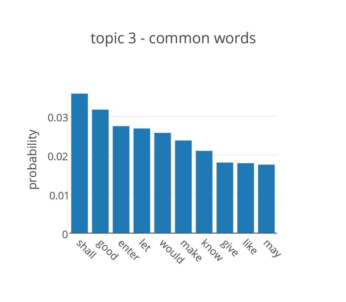
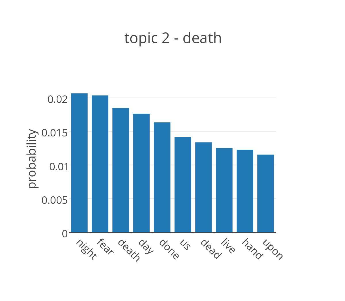
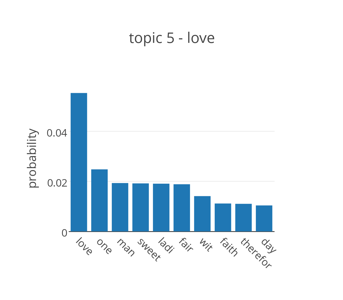
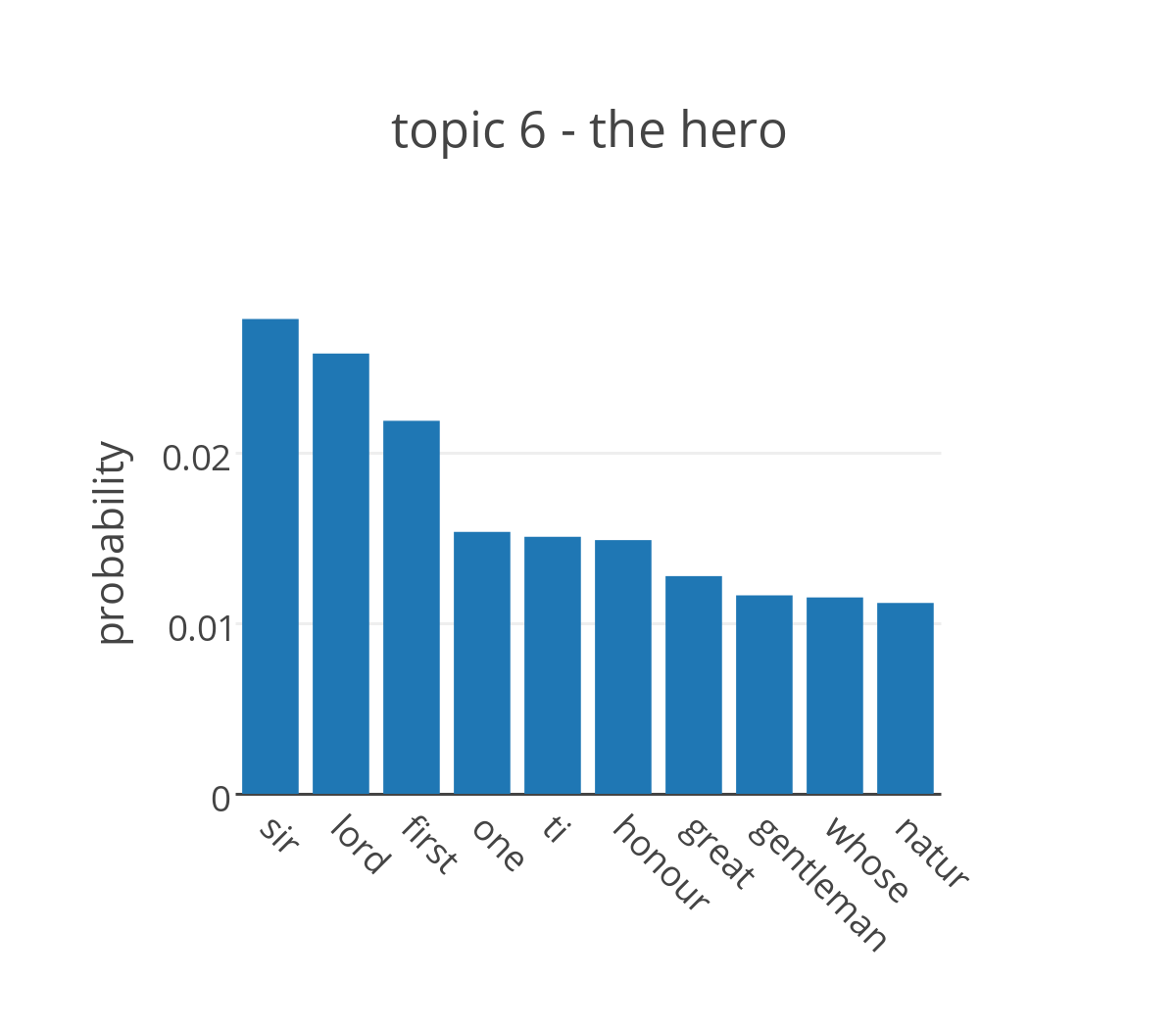
The figure shows the probabilities for the top ten words in four of the topics extracted from the plays. The most likely words to appear in topic 2 are terms that are commonly used in a conversation without adding too much meaning to it, but are generally not included in the list of stop words. It’s not ideal, but it makes sense that they cluster together into a single topic. The top distributions of topics 2, 5, and 6 are more promising and can be easily associated with three of the main themes in Shakespeare’s plays, respectively death, love and the hero.

The other output of LDA is the distribution of topics in the documents.

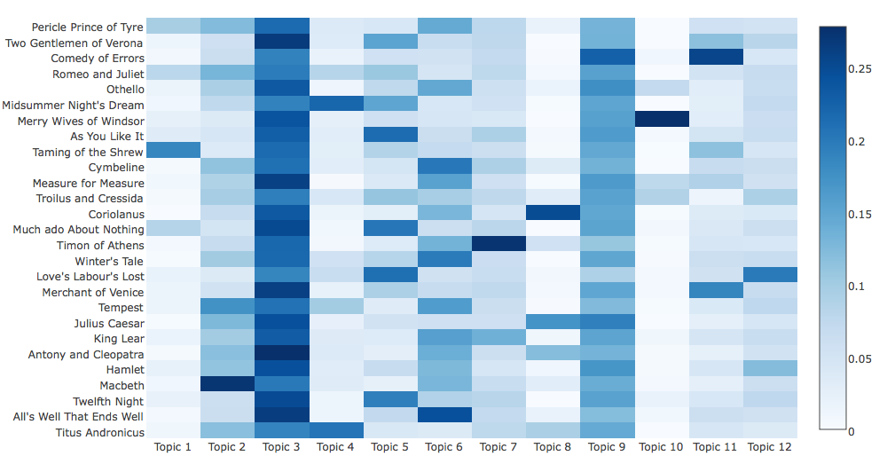
In the figure above, topics are on the x-axis and each line represents a document. Boxes are colored according to the probability of topics in each play: darker blues indicate higher probability of appearing in a specific document and lighter colors indicate lower probabilities. Unsurprisingly, the boxes in the columns of the topics associated with common words (3 and 9) are consistently darker. Since the clustering algorithm aims for a partition that maximizes the differences between groups, these topics will not be very useful in grouping the plays. However, there is enough variability to pass these representations of the documents as input to a clustering algorithm for the grouping.

Step 2: K-Means clustering

K-Means is a simple unsupervised algorithm for solving clustering problems. The goal is to create a partition of n elements into k groups so that each element is assigned to the cluster with the nearest mean. Given an initial set of k means the algorithm assigns each observation to the nearest cluster in terms of Euclidean distance, then recalculates new means to be the averages of the observations in each cluster and reiterates until the assignment no longer changes. At the end of the procedure, elements in the same group are more similar to each other than to elements in different groups.

The topics’ probabilities are the features used as inputs of K-Means. The result is a vector of labels that divides the plays in two groups. In the table, tragedies are highlighted in bold.

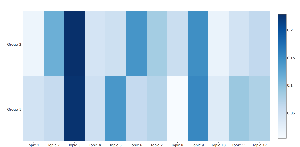
The first group is entirely composed by comedies, except for Romeo and Juliet, while the second group is evenly split between the two categories. This is not a great result. In order to understand the grouping, it is useful to look at the average distributions of the groups. As expected, these show that when a topic is more likely to appear in a group of documents, its probability is lower in the other.

Explaining the results

Content doesn’t seem enough to explain the differences between comedies and tragedies, but it can explain the evolution of Shakespeare’s personal writing style.

When looking at the distribution of the year the plays were first performed the two groups show some overlap around 1600, but it seems clear that the plays in one group were staged significantly earlier than the others.

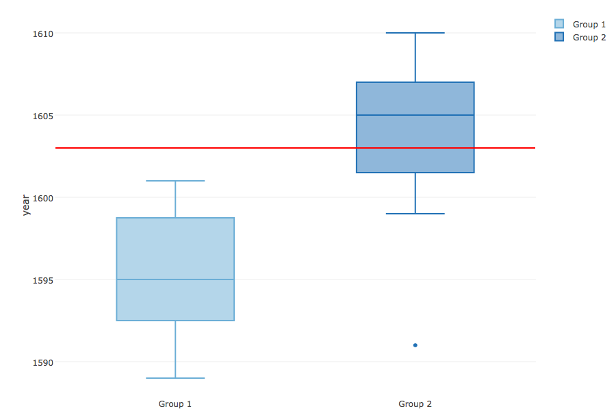
At the time of this analysis I had no idea what this could possibly mean, but the internet is a magical place and has a good explanation for this. The traditional classification of comedies, tragedies, and histories follows the categories of the First Folio, the first complete collection of Shakespeare’s works, published in 1623. Modern critics don’t necessarily agree with it and have introduced different terms and categories. One of the categorizations follows the evolution of Shakespeare’s style over time, identifying an Elizabethan Shakespeare, who is younger and more influenced by the classics, as opposed to a Jacobean one, more mature and writing for a different king. It is not possible to pinpoint exactly when the change happens, but scholars indicate the end of Queen Elizabeth’s reign (1603) and first years of the reign of King James as the time he reaches his maturity, shifting not just the subject of his work but also his style.

Epilogue

It turns out my teachers were right and text analysis does lead to a better understanding of how and why a piece was written. This was a fun exercise (far more fun than writing the essays) and led to some unexpected insight. The thought of machines understanding human languages still blows my mind, but I think I have a better understanding of how NLP works. At least good enough to come up with my own analysis and get some useful information out of a corpus, and that’s a win.

All the analysis is done in Python using the Natural Language Toolkit for text manipulation and scikit-learn and lda packages for the modeling. If you’re interested in the code, there is a repo here: it includes all the inputs, papers and a not-so-messy notebook with all the code used for this article.