A tour of random forests
Random forests are an excellent “out of the box” tool for machine learning with many of the same advantages that have made neural nets so popular. They are able to capture non-linear and non-monotonic functions, are invariant to the scale of input data, are robust to missing values, and do “automatic” feature extraction.
Additionally, they have other benefits that neural nets do not. What follows is a look into how random forests work, how they may be usefully applied, and a discussion of some situations in which they may be preferable to neural networks.
Forest Internals
So how do random forests work? The random forest is an ensemble machine learning model, a composite of many simpler models called decision trees. The individual trees are formed by branching on each of the included features and the random forest is an aggregation of these trees.
Decision Trees
Decision trees branch on each of the included features in order to partition the data. For each bin in the partition (i.e. leaf of the tree), we assign an output value to inputs contained in that bin.
The simple case is a classification problem in which the output is categorical. Suppose, for example, we were attempting to model the effects of cooperation in the classic “prisoner’s dilemma” game. Our decision tree might look something like this (features in circles, outputs are leaves):

Our features are the behavior of each of the prisoners (our outputs are the corresponding prison terms). From the combination of these features we can partition the outcome space into each of the four possible cases.
Slightly more complicated is the case of continuous output. The leaves of the tree will still form a partition of the output space but there are many possible values within each bin. How do we assign a single value? We take the mean among values assigned to that bin.
For example, suppose we have a sample for which the input values are uniformly distributed accross the interval . For each input value, , the corresponding output is . Our decision tree might look something like this:

Given our features, we are able to partition the data into four bins. The output for a given bin is the mean output of the observations contained within it.
There are a few things worth noting here. First, the fact that we can branch on ranges of a continuous value allows us to model non-linear / non-monotonic behaviour. Additionally, it’s straightforward to see that with more features, we can construct a tree with more leaves (a finer partition of the data) and more closely approximate continuous valued output.
Entropy & “Guess Who?”
It’s clear that the order of branches in a decision tree matters. Less transparent is how the path to each leaf is constructed.
This happens according to an iterative approach. For each level of a predetermined depth, we branch on the feature which maximizes the information gain. Information gain is defined in terms of entropy, which is defined as . The information gain of branching on a feature, , is . Thus, at each iteration, we branch on the feature which minimizes the conditional entropy.
Unless you’re reasonably familiar with information theory, the intuition behind this procedure may not be obvious.
A more intuitive way to understand this is the game “Guess Who?”. What questions should we ask to most quickly identify the opposing player’s character (or more formally, given a feature space of all binary classifications, how do we partition the output space with a minimum depth tree)?

It’s typical to ask questions like whether the character “wears glasses” or “has white hair”. But these questions represent features with low information gain; more likely than not, the answer will be no and we will have eliminated only a few possibilities.
A higher information gain feature will partition the data as evenly as possible. Consider a different strategy. “Is your character Connor, or James, or Nick, or Sarah, or Justin, or Tyler, or Ashley, or Kyle, or Joshua, or Megan, or Andy, or Joseph?”

This question represents a feature which perfectly bisects the data; we are guaranteed to eliminate exactly half of the possibilities. And we can repeat this in subsequent iterations. In the general case (of characters), we can identify the target character with only operations.
Trees To Forests
If the unnatural features in our “Guess Who?” example make you nervous about overfitting, you’re not wrong. Overfitting is a well-known pitfall for decision trees. If we add an additional 1000 characters onto the board, asking about the 12 characters from before is a bad question and will almost certainly underperform “white hair”.
This is the purpose of random forests. To avoid overfitting with a single tree, we build an ensemble model through a procedure called bagging.
For some number of trees, , and predetermined depth, , select a random subset of the data (convention is roughly with replacement) and train a decision tree on that data (as discussed above). To train the tree, use a subset of the available features (roughly by convention, where is the total number of features).
Obviously, these parameters can be tuned to fit the needs of the application. A model with more trees / data can take longer to train but may have greater accuracy. More depth / features increases the likelihood of overfitting but may be appropriate if features have complex interactions.
In the case of a classification problem, we use the mode of the trees’ output to classify each value. For regression problems, we use the mean of the output trees. Note that the aggregation process is independent of the internal workings of the individual decision trees. Because each tree can make a prediction using the available features (or a subset thereof), they can be polled to form an aggregate prediction.
It’s difficult to overfit with only a subset of the available information. By building the random forest model as an aggregation of weaker models (weak in that the trees are trained on a subset of the available information) we are able to build a strongly predictive model while avoiding the pitfalls of overfitting.
Some Illustrative Examples
What makes random forests such an effective tool is their robustness to different types of data (e.g. non-linear / non-monotonic functions, un-scaled data, data with missing values, data with poorly chosen features). This makes them an excellent “out of the box” tool for general machine learning problems which do not immediately suggest themselves to a specific alternative.
Take, for example, a function like , where is a random value uniformly distributed in the interval . It’s a “simple” function but it is both non-monotonic and non-linear. A technique like simple regression is a non-starter without significant feature extraction. However, it is a simple task for a random forest.
from sklearn.ensemble import RandomForestRegressor
import numpy as np
import math

def generate_data():
        X, Y = [], []
        f = lambda x : x * math.sin(x) + np.random.uniform()
        for x in np.arange(0, 10, 0.05):
                X.append([x])
                Y.append(f(x))
        return (X, Y)

X, Y = generate_data()
model = RandomForestRegressor()
model = model.fit(X, Y)
This code gives us a model which looks like this.
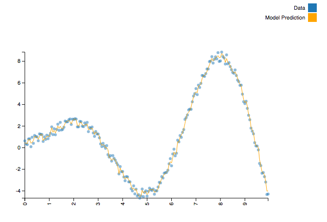
The actual creation of the trained model requires no configuration or feature extraction at all. Said another way, it doesn’t require the practitioner to understand anything about the (complex) shape of the function we’re modeling.
It’s worth noting that other algorithms within “classical” machine learning can accomplish this as well. You could get similar results with k-nearest neighbors or support vector machines. But such approaches fall apart in other common cases such as data with unscaled features (intuitively speaking, models which depend on “distance” will be dominated by features with larger scale).
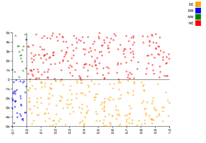
Consider the following example. We will seek to classify points as being within four quadrants: “NE” ( and ), “NW” ( and ), “SE” ( and ), and “SW” ( and ). A straightforward example, except that our values will cover the interval while our values will cover the interval .
import numpy as np
from sklearn.ensemble import RandomForestClassifier
import math

def quadrant(coords):
        EW = 'W' if coords[0] < 0 else 'E'
        NS = 'S' if coords[1] < 0 else 'N'
        return NS + EW

N = 10000
x = -0.1 + np.random.sample(N) * 1.1
y = -5000 + np.random.sample(N) * 10000

xy_coords = list(zip(x, y))
quadrant = list(map(quadrant, xy_coords))

model = RandomForestClassifier()
model = model.fit(xy_coords, quadrant)
This code gives us a classification model which handles the data exactly as intended.
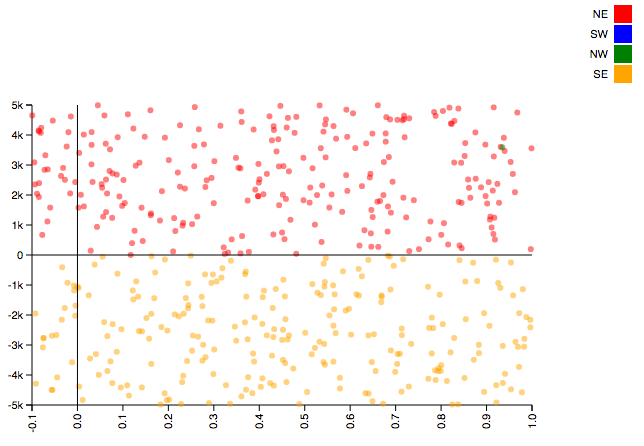
Try to solve the same classification problem with k-nearest neighbors (use a KNeighborsClassifier in place of the RandomForestClassifier) and you will end up with a model like this (support vector machines have similarly dissapointing results).
What About Neural Nets?
In a time when neural networks are as popular as they are, it’s tempting to ask why any of this matters. Why not just use neural nets?
There are several advantages that random forests have over neural networks.
-
Parameter tuning tends to be simpler; there are well established conventions for choosing parameters in random forests but how to determine network layer structure is fairly opaque.
-
There is a more robust body of academic literature around them which makes the internal workings (arguably) easier to understand.
-
Generally simpler to implement. Popular implementations (e.g. scikit-learn) allow users to train sensible random forests with as little as a single line of code. Configuring network layer architecture generally involves more set up.
-
Random forests are extremely well supported for distributed deployment. Through MLlib, random forests are included in Apache Spark and are therefore easily scalable.
With all that said, neural networks do have distinct advtanges. They tend to be even better at automatic extraction of features than forests. They can also be more efficient to train. With nets, there is a global loss function to which gradient descent can be applied; forests must be trained by layers.
The clearest benefit is around predictive performance. The best performing models in many well publicized machine learning challenges tend to be deep neural nets. If incremental gains in model performance are important, this concern may reasonably trump all others.
Ultimately, the choice is application specific. Depending on the details of the problem, one or both of these approaches may be appropriate.
In any case, random forests’ robustness to various types of challenging data and amenability to scaling make them an excellent choice for a large range of applications and a very reasonable first choice for problems that don’t clearly suggest a specific alternative.