A history of storage media

Storage is an essential part of every computer architecture, from the hypothetical paper tape in a Turing machine to the registers and memory unit of the von Neumann architecture. Non-volatile storage media and volatile memory devices have both gone through several technological evolutions over the last century, including some delightfully strange mechanisms. This article is a very selective history, focusing on a handful of the earliest technologies that I find especially interesting:

1. Punch cards, one of the earliest forms of computer data, used for weaving patterns and census data!
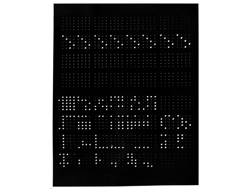
2. Williams-Kilburn tubes, the first electronic memory, where bits were stored as dots on the screen!
3. Mercury delay lines, two-foot-long tubes of hot mercury, which stored bits as pulses of sound!

For a more comprehensive resource, the Computer History Museum has a detailed timeline, featuring lovely photographs. Storage and memory have a rich history. While CPU architectures are quite diverse, they tend to use the same basic elements – switches, in the form of transistors or vacuum tubes, arranged in different configurations. In comparison, the basic components of memory mechanisms have been incredibly varied; each iteration essentially reinvents the wheel.

1. Punch cards

Punch cards aren’t really a strange storage medium, but they are among the earliest, and have had some fascinating historical applications.

1.1. Jacquard looms

Many early ancestors of computers were controlled by punch cards. The ancestor of these machines, in turn, was the Jacqard loom, which automated the production of elaborately woven textiles. It was the first machine to use punch cards as an automated instruction sequence.

First – some background information about weaving patterns into fabric.

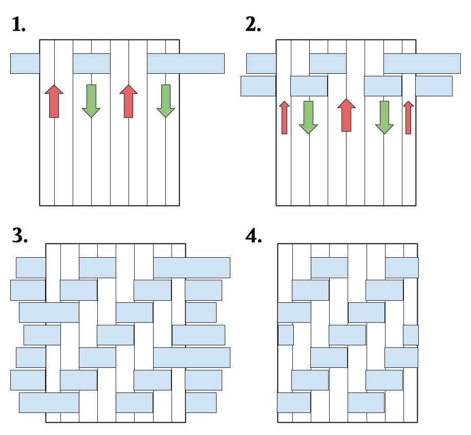
Most fabric is woven with 2 sets of yarn that are perpendicular to each other. The first set of threads, the warp, is stretched out over a loom, and the second set, the weft, is passed either over or under the threads of the warp to form the fabric. This over–under operation is easily represented by binary information. Changing the order of the over–under produces different kinds of fabrics, from satins to twills to brocades.

In the following example of a woven design, the warp is white, and the weft is blue. To form a twill weave, which is what most denims are, the loom raises the first two threads, drops the second two, raises the next two, and so on, across the warp. The weft is then passed between the raised and lowered sets of threads, to weave in the first row. The loom repeats the process, raising alternating sets of warp threads, then passing the weft through. After a few rows¹, the characteristic zigzag pattern of a twill appears.

Although weaving can be very intricate, this particular kind has two simple operations, repeated according to very specific patterns. Computers excel at simple and repetitive work!

Before the Jacquard loom, this process of raising and lowering threads was done by hand on a drawloom. A warp might be about 2000 threads wide, so weaving a detailed pattern in fabric would require making decisions about raising or lowering thousands of threads, thousands of times. Depending on the complexity of the design, an experienced weaving team could weave a few rows every minute, so an inch of fabric would take a day to produce. For context, a ball gown might take up to four yards of decorated fabric, which represents nearly four months of weaving.

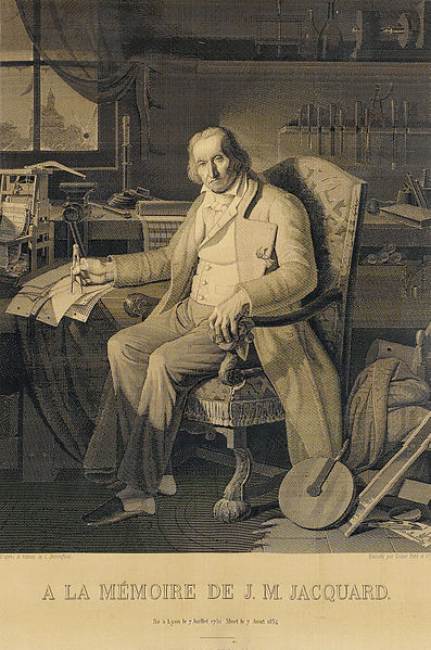
Around 1803, Joseph-Marie Jacquard started building a prototype for a loom that automated the production of decorated cloth. The Jacquard loom wove elaborate silk patterns by reading patterns off a series of replaceable punch cards. The cards that controlled the mechanism could be chained together, so complex patterns of any length could be programmed in.

Twill weaves, like the one above, are fairly easy and repeatable patterns, and they are a trivial example of what an automated loom can produce. The special power of the Jacquard loom comes from its ability to independently control almost every warp end.² This is pretty amazing! A Jacquard mechanism can produce incredibly detailed images. The portrait of Joseph-Marie Jacquard is a stunning demonstration of the intricacy of the loom; the silk textile was woven using tens of thousands of punch cards.

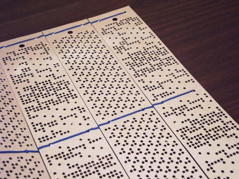
The ability to change the pattern of the loom’s weave simply by changing cards was a conceptual precursor to programmable machines. Instead of a looped, unchanging pattern, any arbitrary design could be woven into the fabric, and the same machine could be used for an infinite set of patterns.

This mechanism inspired many other programmable automatons. Charles Babbage’s Analytical Engine borrowed the idea. In fact, Babbage himself was rumored to have the woven portrait of Jacquard in his house! Player pianos use punch cards (or punched drums) to produce music. That said, most of the early uses of punch cards were for basic, repetitive control of the machines —- simple encodings of music or weaves for specialty use cases. The control languages of the early automatons were limited and not very expressive. The full expressive power of punch cards wasn’t realized until almost 100 years later, when they became the tool for all large-scale information processing.

1.2. The 1890 United States Census

In the late 19th century, the U.S. Census Bureau found itself collecting more information than it could manually process. The 1880 census took over 7 years to process, and it was estimated that the 1890 census would take almost twice as long.³ Spending a decade processing census information meant that the information was obsolete almost immediately after it was produced!

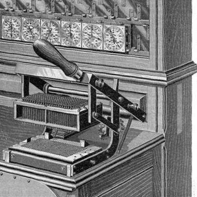
To cope with the growing population, the census bureau held a competition for a more efficient method to count and process the data. Herman Hollerith came up with the idea to represent census information on punched cards, and produced a tabulating machine that could sort and sum the data. His design won the competition, and was used to count the U.S. Census in 1890. The tabulator enabled much faster processing, and provided many more statistics than were available for earlier years.

After the success of the tabulator in the 1890 census, other countries began adopting the technology. Soon, Hollerith’s Tabulating Machine Company produced machines for many other industries. After his death, the Computer Tabulating Recording Company renamed itself to the International Business Machines Corporation, or IBM, leading us into a new era of computing.

Soon after the 1890 census, almost all information processing was done via punch card. By the end of World War I, the army used punch cards to store medical and troop data, insurance companies stored actuarial tables on punch cards, and railroads used them to track operating expenses. Punch cards also became well-established in corporate information processing: throughout the 1970s, punch cards were used in scientific computing, HR departments of large companies, and every use case in between.

Though the once-ubiquitous punch cards have been replaced by other data formats, their echoes are still with us today —- the suggested 80-character line limit for code comes from the IBM 80-column punch card format.

2. Williams-Kilburn Tubes

In the era of punch cards, the cards were mostly used for data while control programs were inputted through complicated system of patch cords. Reprogramming these machines was a multi-person, multi-day undertaking! To speed up this process, researchers proposed using easily replaceable storage mechanisms for storing both programs and data.

While it’s possible to build computers using mechanical memory, most mechanical memory systems are slow and tediously intricate. Developing electronic memory for stored-program computing was the next big frontier in computer design.

In the late 1940s, researchers at Manchester University developed the first electronic computer memory, essentially by cobbling together surplus World War II radar parts. By making a few ingenious modifications to a cathode ray tube, Frederic Williams’ and Tom Kilburn’s lab at Manchester built the first stored-program computer.

During the Second World War, cathode ray tubes (CRTs) became standard in radar systems, which jump-started research into more advanced CRT technology. Researchers at Bell Labs took advantage of a few secondary effects of cathode ray tubes to use the tubes themselves to store the location of past images. Williams and Kilburn took the Bell Labs work a step further, adapting the CRTs for use as digital memory.

2.1. Secondary effects: principles of operation

The Williams-Kilburn tube turned spare parts from radar research and a few side effects of CRT tubes into the first digital memory.

A conventional CRT displays an image by firing an electron beam at a phosphorescent screen. Electrostatic plates or magnetic coils⁴ steer the beam, scanning across the entire screen. The electron beam switches on and off to draw out images on the screen.

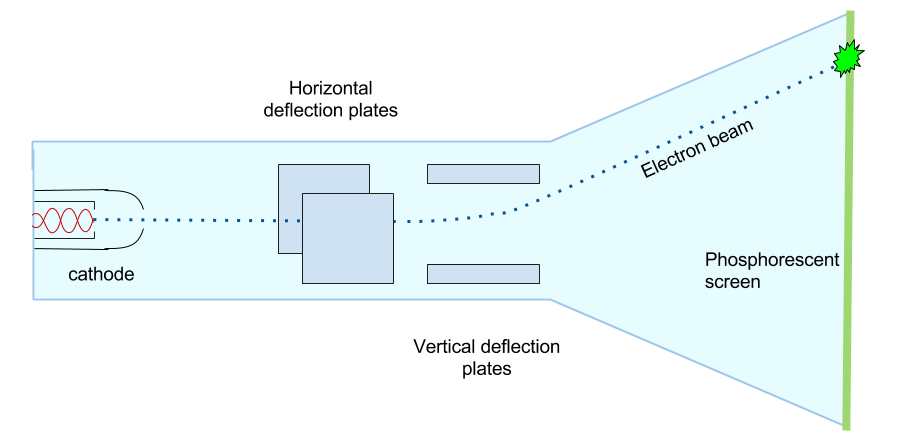
Depending on the type of phosphor on the screen and the energy of the electron beam, the bright spot lasts from microseconds to several seconds. During normal operation, once written, the bright spot on the screen can’t be detected again electronically.

However, if the energy of the electron beam is above a specific threshold, the beam knocks a few electrons out of the phosphor, an effect called secondary emission. The electrons fall a short distance away from the bright spot, leaving a charged bullseye that persists for a little while.

Thus, to write data, Williams-Kilburn tubes use a high-energy electron beam to charge spots on the phosphor screen. Bits of storage are laid out in a grid across the face of the tube, much like pixels on a screen. To store data, the beam sweeps across the face of the tube, turning on and off to represent the binary data. The charged areas across the screen are essentially little charged capacitors.

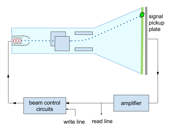
When the higher energy electron beam hits the screen, the secondary emission of electrons induces a small voltage in any conductors near it. If a thin metal sheet is placed in front of the CRT’s phosphor screen, the electron beam knocks a few electrons out of the phosphor screen, inducing a voltage change in the metal sheet, as well.

Thus, to read data, the electron beam again sweeps across the face of the tube, but stays on at a lower energy. If there were a ‘1’ written there already, the point of positive charge on the screen gets neutralized, discharging the capacitor. The pickup screen then sends a pulse of current. If there were a ‘0’, no discharge occurs, and the pickup plate sees no pulse. By noting the pattern of current that comes through the pickup plate, the tube can determine what bit was stored in the register.⁵ The Williams tube was true random access memory – the electron beam could scan to any point in the screen to access data near-instantly.

The charge of areas leak away over time, so a refresh/rewrite process is necessary. Modern DRAM has a similar memory refresh procedure, too! Since the read is destructive, every read is followed by a write to refresh the data.

The data in a Williams-Kilburn tube could be transferred to a regular CRT display tube for scrutiny, which was great for debugging. Kilburn also reported that it was quite mesmerizing to watch the tube flicker as these early machines computed away.

2.2. The Manchester Baby

After the team at Manchester had a working memory tube that stored 1024 bits, they wanted to test the system in a proof-of-concept computer. They had a tube that would store data written to it manually, at slow speeds, but they wanted to ensure that the whole system would still work at electronic speeds under a heavy write load. They built the Small Scale Experimental Machine (a.k.a. the Manchester Baby) as a test bed. This would be the world’s first stored-program computer!

The Baby had four cathode ray tubes:

• one for storing 32 32-bit words of RAM,
• one as a register for an accumulator,
• one for storing the program counter and current instruction,
• one for displaying the output or the contents of any of the other tubes.

Williams-Kilburn tubes are an unusually introspectable data storage device.

Programs were entered one 32-bit word at a time, where each word was either an instruction or data to be manipulated. These words were inputted by manually setting a set of 32 switches to on or off! The first program that was run on the Manchester Baby calculated factors for large numbers. Later, Turing wrote a program that did long division, since the hardware could only do subtraction and negation.

2.3. Later history

Parts from the Manchester Baby were repurposed for the Manchester Mark 1, which was a larger and more functional stored-program computer. The Mark 1 developed into the Ferranti Mark 1, which was the first commercially available general-purpose computer.

The Williams-Kilburn tube was used as RAM and storage in a number of other early computers. The MANIAC computer, which did hydrogen bomb design calculations at Los Alamos, used forty Williams-Kilburn tubes to store 1024 40-bit numbers.

Though the tubes played a large part in early computer history, they were quite difficult to maintain and run. They frequently had to be tuned by hand, and were eventually phased out in favor of core memory.

3. Mercury Delay Lines

In addition to Williams-Kilburn tubes, radar research yielded another memory mechanism for early computers – delay line memory. Defensive radar systems in the 1940s used primitive delay lines to remember and filter out non-moving objects at ground level, like buildings and telephone poles. This way the radar systems would only show new, moving objects.

Delay lines are a form of sequential access memory, where the data can only be read in a particular order. A vertical drainpipe can be a simple delay line – you push a ball with data written on it in one end, let it fall through the pipe, read it, then throw it back in the other end. Eventually, you can juggle many such bits of data through the pipe. To read a particular bit, you let the balls fall and cycle through until you reach the bit you want. Sequential access!

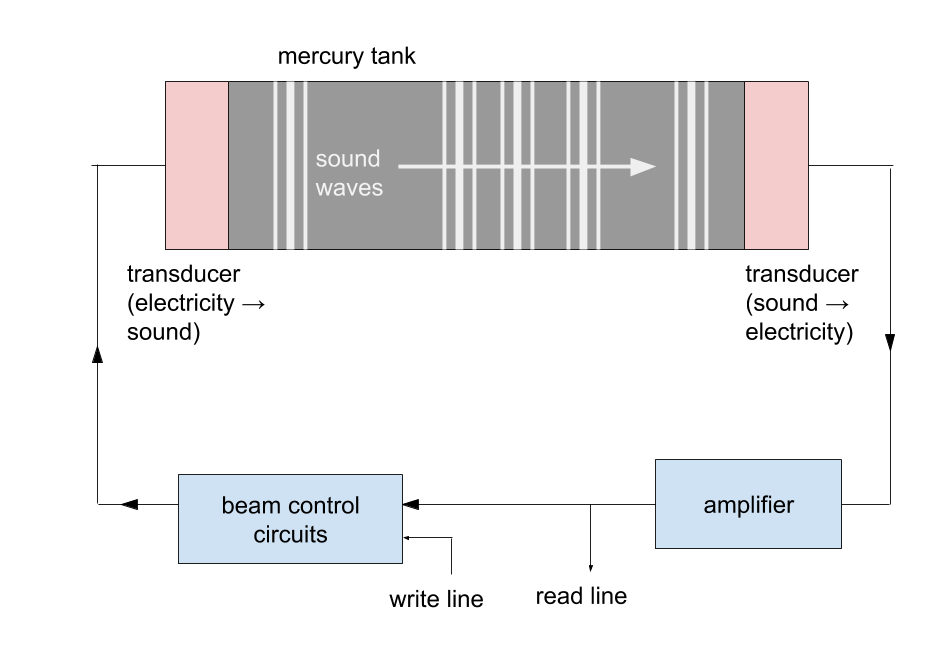
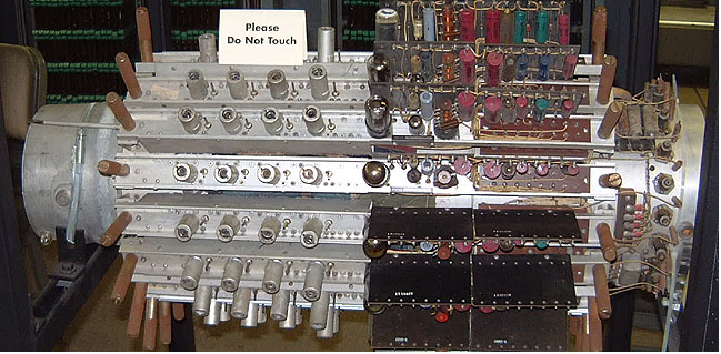
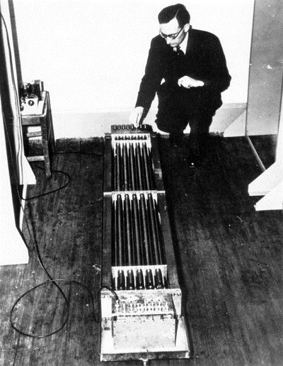
The most common form of delay lines in early computers was the mercury delay line. This was essentially a two-foot-long pipe filled with mercury, with a speaker on one end, and a microphone on the other (in practice, these were identical piezoelectric crystals). To write a bit, the speaker would send a pulse through the tube. The pulse would travel down the tube in half a millisecond, where it would be read by the microphone. To keep the bits stored, the the speaker would then retransmit the bits just read back through the tube. Like the drainpipe example, to read a particular bit, the circuitry had to wait for the pulse it wanted to cycle through the system.

Mercury was chosen because its acoustic impedance at 40ºC (104ºF) closely matched the piezoelectric crystals used as transducers. This reduces echoes that might interfere with the data signals. At this temperature, the speed of sound in mercury is about four times that in air, so a bit passes through a 2-foot-long tube in about 420 microseconds. Since the computer’s clock needs to be kept exactly in line with the memory cycles, keeping the tube at exactly 40ºC was critical.

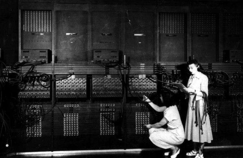
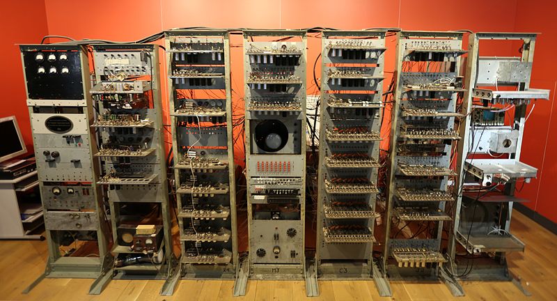
While the Manchester Baby was the first stored-program computer, it was only ever meant as a proof-of-concept. EDVAC, built for the U.S. Army, was the first practically used stored-program computer. John von Neumann’s report on EDVAC inspired the design many other stored program computers.

So, mercury delay lines were giant tubes of liquid mercury, kept in ovens at 40ºC, cycling bits of memory through as sound waves! Despite their unwieldiness, mercury delay lines were used in a number of other early computers. EDSAC, which was inspired by von Neumann’s report, was the first computer used for computational biology, and was also the computer on which the first video game was developed (a version of tic-tac-toe with a CRT display). UNIVAC I, which was the first commercially available computer, also used mercury delay lines. The first UNIVAC was installed at the U.S. Census Bureau in 1951, where it replaced an IBM punch card machine. It was eventually retired in 1963.

And more!

This is just the story of the first few memory mechanisms that came on the market; other unique mechanisms have been developed in the decades since delay lines. Soon after, core memory – ferrite donuts woven into mats of copper wire – became ubiquitous. A read-only version of core memory was on the Apollo Guidance Computer, which took astronauts to the moon. Until a few years ago, nearly every computer had several spinning platters coated in a thin layer of iron, carefully magnetized by a needle hovering over a cushion of air. For years, we passed data and software around on plastic disks covered in little pits, read by bouncing a laser off the surface. Fancier disks, which can store up to 25 GB of data, use blue lasers, instead.

Computers are incredible Rube Goldberg machines – each layer is made of fractal complexity, carefully hidden away behind layers of abstraction. Examining the history of the technology gives us some insight into why the interfaces look the way they do now, and why we use the terminology we do. Early computing history produced a bestiary of fascinating and complicated memory devices. Each system is an incredibly well-engineered piece of machinery that leaves its imprint on computers to come.

Parts of this article originally appeared on Kiran’s blog.