Image Processing 101

Why this was written

At the Recurse Center, I spent some time teaching myself image processing. When I started, I had no idea what it entailed. I just knew that it could help me recognize text, shapes and patterns and to do interesting things with them.

My sources have mainly been Wikipedia pages, books and publicly available university lecture notes. As I became more familiar with the material, I wished for an ‘Image Processing 101’ article that could give anyone a gentle introduction to the world of image processing.

This is my attempt at writing that article.

Prerequisites

This article is designed for those who are comfortable with Python. No other previous knowledge is required, although some familiarity with numpy and matrix operations will be helpful.

Getting started

We’ll be using OpenCV for Python, Python 2.7¹, and iPython Notebook. For instructions on how to set up OpenCV on MacOS, there are instructions here.

All code and images used are available as a runnable iPython notebook on Github. You can also see the iPython notebook online.

I highly recommend learning image processing work on iPython notebook as it allows you to display images inline, which makes it really easy to get feedback on what your code is actually doing.

What is image processing?

Image processing is the process of manipulating or performing operations on images to achieve a certain effect (making an image grayscale, for example), or of getting some information out of an image with a computer (like counting the number of circles in it).

Image processing is also very closely related to computer vision, and we do blur the line between them a lot. Don’t worry too much about that – you just need to remember that we are going to learn about methods of manipulating images, and how we can use those methods to collect information about them.

In this article, I will go through some basic building blocks of image processing, and share some code and approaches to basic how-tos. All code written is in Python and uses OpenCV, a powerful image processing and computer vision library.

Building blocks

Let’s start off with the imports. We’re using cv2, numpy and a little bit of matplotlib (mostly as a convenient way of displaying images).

import cv2, matplotlib
import numpy as np
import matplotlib.pyplot as plt

Image format

Alright! Let’s get started. Firstly, we’ll need to read in images and to understand the format in which they are represented to us.

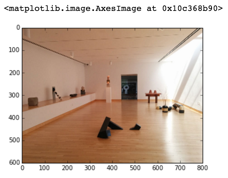
In OpenCV, images are represented as 3-dimensional Numpy arrays. An image consists of rows of pixels, and each pixel is represented by an array of values representing its color.

Given an image above, the array representation of it will be:

# read an image
img = cv2.imread('images/noguchi02.jpg')

# show image format (basically a 3-d array of pixel color info, in BGR format)
print(img)

Results:

[
    [[72 99 143]   [76 103 147]  [78 106 147]  ...,   [159 186 207]  [160 187 213]  [157 187 212]]
    [[74 101 145]  [77 104 148]  [77 105 146]  ...,   [160 187 208]  [158 186 210]  [153 183 208]]
    [[76 103 147]  [77 104 148]  [76 104 145]  ...,   [157 181 203]  [160 188 212]  [158 186 210]]
    ...,
    [[39 78 130]  [39 78 130]  [40 79 131]  ...,   [193 210 223]  [195 212 225]  [197 214 227]]
    [[32 71 123]  [32 71 123]  [32 71 123]  ...,   [198 215 228]  [200 217 230]  [200 217 230]]
    [[39 78 130]  [39 78 130]  [39 78 130]  ...,   [199 216 229]  [200 217 230]  [201 218 231]]
]

Where [72 99 143], etc., are the blue, green, and red (BGR) values of that one pixel. Note that OpenCV loads an image in BGR format by default. Matplotlib, however, reads in images as RGB. To display an image in matplotlib, we will need to convert the BGR format to RGB. I’ll let you figure out what happens when you forget to do the conversion before passing the image in to matplotlib.

# convert image to RGB color for matplotlib
img = cv2.cvtColor(img, cv2.COLOR_BGR2RGB)

# show image with matplotlib
plt.imshow(img)

Colors

Wait, hold up, hold up. What’s the reason for all this business with BGR and RGB?

Red, Green and Blue (RGB)

In the digital world, colors are commonly represented using the RGB color model. By this color model, red, green and blue light can be added together in various ways to produce a range of colors on the visible spectrum. Each one of thse colors are referred to as a channel. This works slightly differently than, say, mixing paint colors. In the RGB color model:

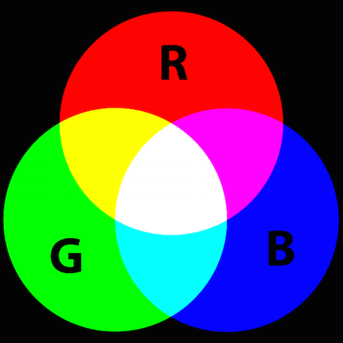Image from Wikipedia ³

• red + green = yellow
• blue + green = cyan
• red + blue = magenta
• red + blue + green = white

I won’t go too much into the technicalities, but Wikipedia has a section on how the color combinations work.

On most systems, RGB values are represented as values ranging from 0 to 255, with higher values corresponding to a higher intensity of that color channel. For example, we can guess that [255, 51, 0] is probably a reddish color, because its R channel is the highest, and that [51, 102, 0] is probaby a greenish color, with the G channel being the highest.

Hue, Saturation and Value (HSV)

Another useful color model is the HSV color model. Instead of representing colors by the red, green and blueness of it, we represent them by the hue (where it is on the range of the rainbow), saturation (the ‘colorfulness’ of the color) and value (also known as brightness, or how much perceived light is coming out of it).

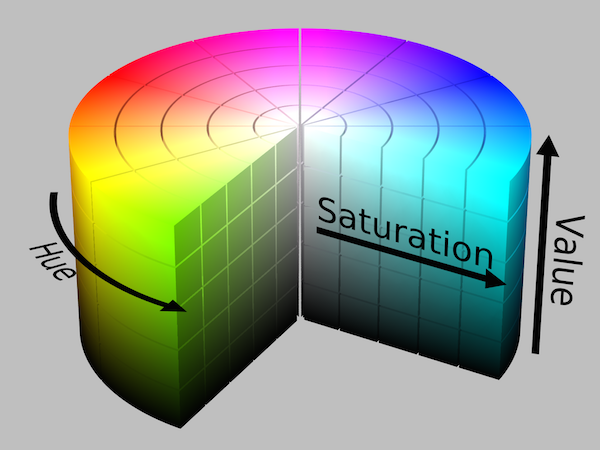Image from Wikipedia ⁴

The HSV color model is especially useful when you want to think of an image’s color in either one of those channels, e.g. looking for parts of an image that fall in the blue hue range.

A variation of the HSV is the HSL color model, which consists of the hue, saturation and lightness. It is similar to HSV, but differs in the definition of saturation and the third channel (value vs lightness)².

Grayscale

We will also be working with grayscale images. Grayscale images only have one color channel on the scale of 0 to 255, representing the brightness of that pixel, with 0 being totally dark (black) and 255 being totally bright (white).

Converting the image we have into grayscale gives us this 2-dimensional array:

# convert image to grayscale
gray_img = cv2.cvtColor(img, cv2.COLOR_RGB2GRAY)

# grayscale image represented as a 2-d array
print(gray_img)

Result:

[[109 113 115 ..., 189 192 191]
 [111 114 114 ..., 190 190 187]
 [113 114 113 ..., 185 192 190]
 ...,
 [ 89  89  90 ..., 212 214 216]
 [ 82  82  82 ..., 217 219 219]
 [ 89  89  89 ..., 218 219 220]]

I recommend playing around with a color picker to get a better idea of how colors vary as you change them around. It’s especially interesting to see how RGB values change as you modify one of the HSV channels.

Exercise:

Knowing this, we can now find the average color of an image! If we averaged each of the R, G and B channels, it will give us an RGB value that is the average pixel color. Here’s an example of how it can be done with np.average().

# find average per row, assuming image is already in the RGB format.
# np.average() takes in an axis argument which finds the average across that axis.
average_color_per_row = np.average(img, axis=0)
​
# find average across average per row
average_color = np.average(average_color_per_row, axis=0)
​
# convert back to uint8
average_color = np.uint8(average_color)
print(average_color)

Result:

[179 146 123]

In order to display a color on matplotlb, we need to create a small 100x100 pixel image populated with that RGB value.

# create 100 x 100 pixel image with average color value
average_color_img = np.array([[average_color]*100]*100, np.uint8)

plt.imshow(average_color_img)

What is the average color of the image?

Segmentation

When we’re trying to gather information about an image, we’ll first need to break it up into the features we are interested in. This is called segmentation. Image segmentation is the process representing an image in segments to make it more meaningful for easier to analyze³.

Thresholding

One of the simplest ways of segmenting an image is thresholding. The basic idea of thresholding is to replace each pixel in an image with a white pixel if a channel value of that pixel exceeds a certain threshold, and a black pixel if it doesn’t. We typically convert an image into a binary image, i.e. a single channel image. Grayscale images are examples of single channel images.

# threshold for image, with threshold 60
_, threshold_img = cv2.threshold(gray_img, 60, 255, cv2.THRESH_BINARY)

# show image
threshold_img = cv2.cvtColor(threshold_img, cv2.COLOR_GRAY2RGB)
plt.imshow(threshold_img)

Result:

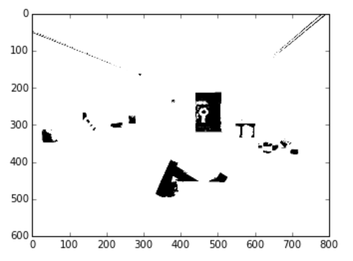
This makes it easy to single out parts of the image that are of different brightness. This doesn’t only have to apply to grayscale versions of images. We can also segment out parts of images by color channels. Color thresholding works best with HSV. We talked about how HSV has a hue channel, that is, on the scale from red to green to blue to magenta, where does the color of the pixel lie?

Rather than finding the value that is under a threshold, we can find parts of the image with hues that lie within a range with cv2.inRange().

# open new Mondrian Piet painting photo
piet = cv2.imread('images/piet.png')
piet_hsv = cv2.cvtColor(piet, cv2.COLOR_BGR2HSV)

# threshold for hue channel in blue range
blue_min = np.array([100, 100, 100], np.uint8)
blue_max = np.array([140, 255, 255], np.uint8)
threshold_blue_img = cv2.inRange(piet_hsv, blue_min, blue_max)

threshold_blue_img = cv2.cvtColor(threshold_blue_img, cv2.COLOR_GRAY2RGB)

plt.imshow(threshold_blue_img)

Result:

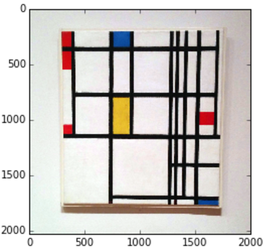Original image

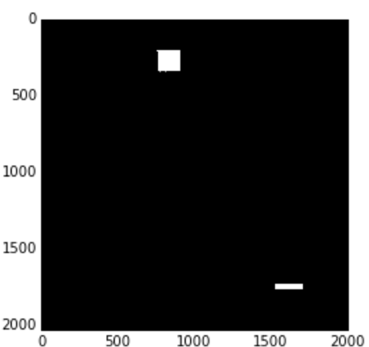Blue hue threshold

Exercise: How would we extract the red or yellow parts of this painting? What ranges do we use for reds or yellows if the entire hue of colors is represented on a scale of 0 to 255?

Masking with a binary threshold

Now that we can identify colors, we can do interesting things like using the binary image as a mask. A mask is a matrix of zero and non-zero values used for a bitwise operation. Masks can be used to cut, or ‘mask’, out certain sections of an image. A mask is usually a matrix of zeros (for the parts to exclude) and non-zeros (for the parts we want to keep).

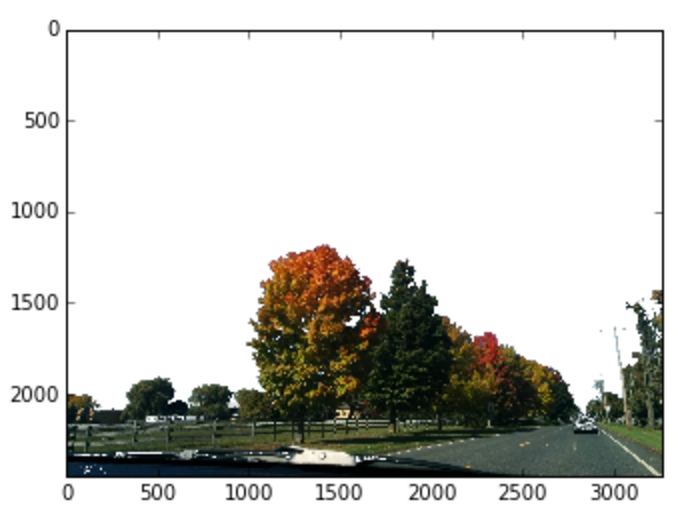
Let’s say I would like a version of an image of an outdoor landscape that excludes the sky. We can first find the pixels that are within range of the blue hue, which will identify the blue-sky parts of an image. To get the parts of the image that are not the sky, we can inverse the values with a bitwise_not, which leaves us the parts that are not blue, giving us our mask. Performing a bitwise_and on that mask with an image will leave only the parts that are not blue.

upstate = cv2.imread('images/upstate-ny.jpg')
upstate_hsv = cv2.cvtColor(upstate, cv2.COLOR_BGR2HSV)
plt.imshow(cv2.cvtColor(upstate_hsv, cv2.COLOR_HSV2RGB))

# get mask of pixels that are in blue range
mask_inverse = cv2.inRange(upstate_hsv, blue_min, blue_max)

# inverse mask to get parts that are not blue
mask = cv2.bitwise_not(mask_inverse)
plt.imshow(cv2.cvtColor(mask, cv2.COLOR_GRAY2RGB))

# convert single channel mask back into 3 channels
mask_rgb = cv2.cvtColor(mask, cv2.COLOR_GRAY2RGB)

# perform bitwise and on mask to obtain cut-out image that is not blue
masked_upstate = cv2.bitwise_and(upstate, mask_rgb)

# replace the cut-out parts with white
masked_replace_white = cv2.addWeighted(masked_upstate, 1, \
                                       cv2.cvtColor(mask_inverse, cv2.COLOR_GRAY2RGB), 1, 0)

plt.imshow(cv2.cvtColor(masked_replace_white, cv2.COLOR_BGR2RGB))

Results :

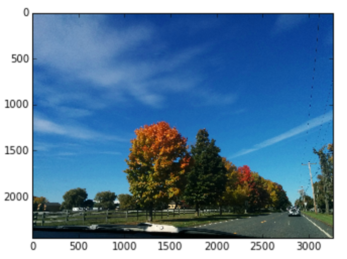Original image

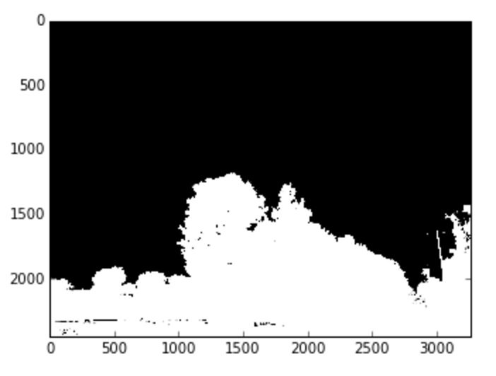Thresholded (mask)

Masked image

Further reading

• For more information about different types of more robust thresholdings and how they work, check out the OpenCV3 documentation.

Blurring

Photographs can be quite noisy, which means there can be small irregularities that may get in the way of image segmenting. A common way to get rid of the noisy bits is to preprocess the image with a Gaussian blur. You can think of blurring as a way of smoothing out high intensities or drastic changes between pixels.

Gaussian blurs work by applying transformations to each pixel in an image. This is done by convolving an image with an n x n-sized kernel. You can think of a convolution as an act of applying an operation on a pixel depending to the values of the n x n pixels around it. The operation is defined by the kernel. So on a Gaussian blur with a 5 x 5 kernel, for every pixel, the 5 x 5 surrounding pixels are considered, and an averaging calculation is performed that will give us the pixels’ new, blurred color. The bigger the Gaussian kernel size, the more blurred the image will be.

img = cv2.imread('images/oy.jpg')

# gaussian blurring with a 5x5 kernel
img_blur_small = cv2.GaussianBlur(img, (5,5), 0)

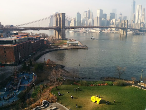Original image (600px by 450px)

Blur with 5x5 kernel

Blur with 15x15 kernel

Gaussian blurring is especially useful when you have a noisy image and would like to smooth over all of those irregularities before performing a thresholding.

Results:

Thresholded original image

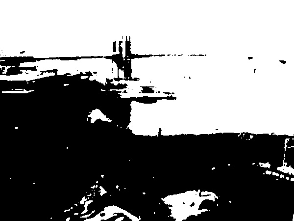Thresholded 5x5 kernel-blurred image

Above is an example of performing a threshold on the unblurred image versus the one blurred by a 5x5 kernel. Blurring gives us cleaner lines on our thresholded portions, which make them easier to work with.

Further reading

• Gaussian Blurring explained on Wikipedia
• Smoothing images explained on OpenCV

Contours and Bounding Rectangles

Now that we have simplified, binary versions of those images, we can use them to identify features of interest. As an example, let’s look at how we can identify the individual coins in an image.

In this section, we will see how we can use contours and bounding rectangles to segment out features.

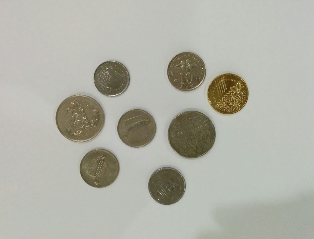Original image

Preprocess image

First, we’ll convert the image to grayscale and will perform a Gaussian blur on it to simplify it and to remove noise. This is a common form of preprocessing, and if often the first step in working with an image.

Then, we’ll perform a binary threshold on the preprocessed image. Since the coins are on a light background, the threshold will pick up the lighter background as the feature of interest. We’ll invert the binary image to pick up the coins.

# get binary image and apply Gaussian blur
coins = cv2.imread('images/coins.jpg')
coins_gray = cv2.cvtColor(coins, cv2.COLOR_BGR2GRAY)
coins_preprocessed = cv2.GaussianBlur(coins_gray, (5, 5), 0)

# get binary image
_, coins_binary = cv2.threshold(coins_preprocessed, 130, 255, cv2.THRESH_BINARY)

# invert image to get coins
coins_binary = cv2.bitwise_not(coins_binary)

Results:

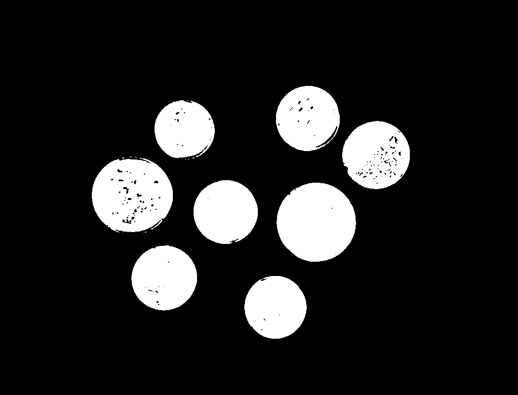Preprocessed binary image

Find contours

Contours are curves joining all the continuous points that have the same color or intensity along a boundary. They’re useful for object or feature detection as well as shape analysis⁴. Using cv2.findContours(), we’ll find the contour of each coin. Passing in the cv2.RETR_EXTERNAL flag to the function returns only the external contours, so it won’t pick up contours for the smaller details on the coin surface.

From those contours, we’ll find the area of each, and filter out the ones that are too small to be coins. Images from real life are rarely perfect, and checks like this are often necessary to filter out noise and outliers. To obtain the area of the contour, we’re using cv2.contourArea().

# find contours
coins_contours, _ = cv2.findContours(coins_binary, cv2.RETR_EXTERNAL, cv2.CHAIN_APPROX_SIMPLE)

# make copy of image
coins_and_contours = np.copy(coins)

# find contours of large enough area
min_coin_area = 60
large_contours = [cnt for cnt in coins_contours if cv2.contourArea(cnt) > min_coin_area]

# draw contours
cv2.drawContours(coins_and_contours, large_contours, -1, (255,0,0))

# print number of contours
print('number of coins: %d' % len(large_contours))

number of coins: 8

Results:

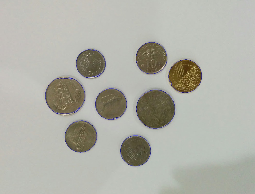Contours of coins from binary image

Find bounding rectangles

A bounding rectangle is the smallest rectangle that can contain a contour. We can use them to segment out individual coins in our image. Do note that the cv2.boundingRect() method returns the bounding rectangle as x and y coordinates of the top left corner of the rectangle, and its width and height. We can also use bounding rectangles to crop out the eight individual coins.

# create copy of image to draw bounding boxes
bounding_img = np.copy(coins)

# for each contour find bounding box and draw rectangle
for contour in large_contours:
    x, y, w, h = cv2.boundingRect(contour)
    cv2.rectangle(bounding_img, (x, y), (x + w, y + h), (0, 255, 0), 3)

Results:

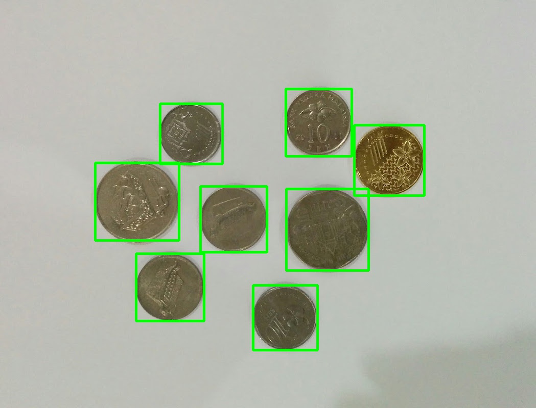Bounding boxes of contours

Further reading

• Understanding contours and contour hierarchy
• Other types of contour features, including contour area and bounding rectangles

Edge detection

Sometimes segmenting via color or intensity as we did with binary thresholding isn’t sufficient. What if we needed to segment out a multicolored object? Think about a blue and yellow striped bowl under non-uniform light – its color is not uniform throughout.

In comes edge detection, a way of finding edges in an image. Edges are defined as points in an image where there is a change in brightness or intensity, which usually means a boundary between different objects. Edge detection is a fundamental part of image processing and is often a starting point for detecting and working with features⁵.

There is quite a bit of math behind edge detection, but we won’t go into that here. The basic idea behind edge detection is that we can measure changes in the brightness of areas of an image, which we call the gradient. We can measure both the magnitude (how drastic the change is) and direction of a gradient. If the magnitude of change at a set of points exceeds a given threshold, then it can be considered an edge.

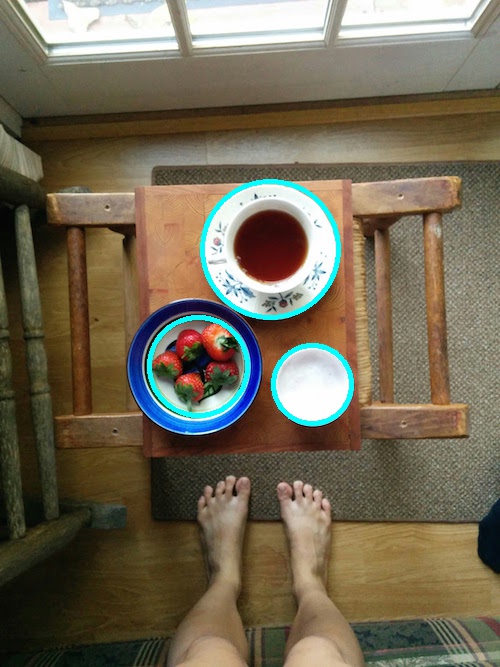
The Canny edge detection algorithm is a popular edge detection algorithm that produces accurate, clean edges. Below is an example of its OpenCV implementation in action, compared to a binary threshold of the same image. Note that the non-uniform lighting on the image makes it impossible to pick out both the bowl and cups with simple thresholding.

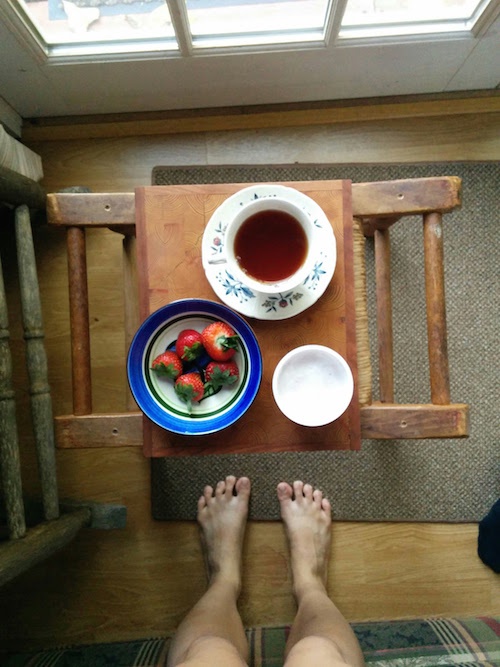Original image

Binary threshold

As standard practice, we’ll preprocess the image with grayscaling and blurring before performing the thresholding. Note how the topmost teacup cannot be captured with simple thresholding. Even if we adjust the threshold value to be much higher to capture the teacup, it will exclude the bowl.

cups = cv2.imread('images/cups.jpg')

# preprocess by blurring and grayscale
cups_preprocessed  = cv2.cvtColor(cv2.GaussianBlur(cups, (7,7), 0), cv2.COLOR_BGR2GRAY)

# find binary image with thresholding
_, cups_thresh = cv2.threshold(cups_preprocessed, 80, 255, cv2.THRESH_BINARY)
plt.imshow(cv2.cvtColor(cups_thresh, cv2.COLOR_GRAY2RGB))

Results:

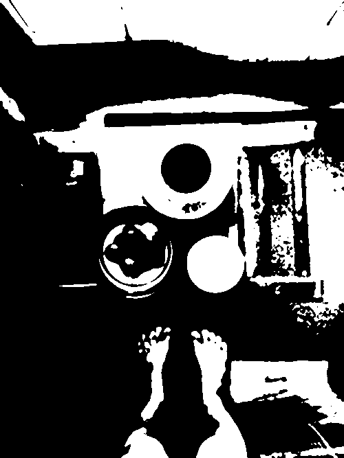Binary image with threshold value of 80. Teacup not captured.

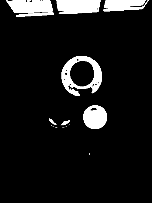Binary image with threshold value of 200. Teacup captured, but not the bowl.

Canny edges

Instead of thresholding, let’s perform Canny edge detection on the image. Note that the cv2.Canny() function takes in two thresholds – the algorithm does what is called double thresholding. If the gradient magnitude is higher than threshold2, it is accepted as a strong edge. If it is lower than threshold2 but higher than threshold1, it will also be considered an edge, albeit a weak one if it is connected to another strong edge.

# find binary image with edges
cups_edges = cv2.Canny(cups_preprocessed, threshold1=90, threshold2=110)
plt.imshow(cv2.cvtColor(cups_edges, cv2.COLOR_GRAY2RGB))
cv2.imwrite('cups-edges.jpg', cups_edges)

Results:

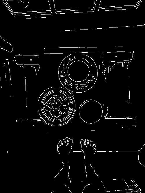Canny edges detected

Canny edge detection does a much better job at picking out features of an image that are otherwise not detected by a simple binary threshold.

Edges are pretty cool and make for interesting effects, but what can do with them?

Line and shape detection

If our objects of interest are of regular shapes like lines and circles, we can use Hough Transforms to detect them.

Line Detection

The Hough Line Transform works by coming up with a list of probable lines that points can be on, where each line is defined in polar coordinate terms of r and theta as r = x * cos (theta) + y * sin (theta). If a probable line has enough other points on it, then it is considered a line.

Here is an example of the Hough Line Transform in action.

# copy of image to draw lines
cups_lines = np.copy(cups)

# find hough lines
num_pix_threshold = 110 # minimum number of pixels that must be on a line
lines = cv2.HoughLines(cups_edges, 1, np.pi/180, num_pix_threshold)

for rho, theta in lines[0]:
    # convert line equation into start and end points of line
    a = np.cos(theta)
    b = np.sin(theta)
    x0 = a * rho
    y0 = b * rho

    x1 = int(x0 + 1000*(-b))
    y1 = int(y0 + 1000*(a))

    x2 = int(x0 - 1000*(-b))
    y2 = int(y0 - 1000*(a))

    cv2.line(cups_lines, (x1,y1), (x2,y2), (0,0,255), 1)

Results:

Edges

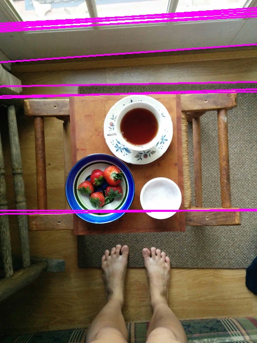Straight lines detected from edges

Circle Detection

The Circle Hough Transform works similarly, but searches for all a, b, and r values that make for possible circles where circles are defined as ( x - a ) ^ 2 + ( y - b ) ^ 2 = r ^ 2. As they have extremely large search spaces, we should ideally set boundaries for the search space (e.g. setting minimum or maximum radius values).

Here is an example of the Circle Hough Transform in action:

# find hough circles
circles = cv2.HoughCircles(cups_edges, cv2.cv.CV_HOUGH_GRADIENT, dp=1.5, minDist=50, minRadius=20, maxRadius=130)
cups_circles = np.copy(cups)

# if circles are detected, draw them
if circles is not None and len(circles) > 0:
    # note: cv2.HoughCircles returns circles nested in an array.
    # the OpenCV documentation does not explain this return value format
    circles = circles[0]
    for (x, y, r) in circles:
        x, y, r = int(x), int(y), int(r)
        cv2.circle(cups_circles, (x, y), r, (255, 255, 0), 4)
    plt.imshow(cv2.cvtColor(cups_circles, cv2.COLOR_BGR2RGB))

print('number of circles detected: %d' % len(circles[0]))

number of circles detected: 3

Results:

Edges

Circles detected from edges

Note that only one circle is detected for the bowl, as we specified that the minimum distance, minDist between circles must be at least 50 pixels.

Further Reading

• Hough transforms explained and demonstrated on OpenCV documentation

What next?

Cool! Now that you know some of the basics, you should hopefully be in a good place to start thinking about your own image processing projects. And even if you don’t have a project in mind, just playing around with the different OpenCV features with different parameters is great way to familiarize yourself with it further.

If you’d like to delve deeper to how these features work (e.g. how does edge detection actually happen?), implementing them in a language of your choice can be a rewarding learning experience. For example, I didn’t fully understand edge detection until I worked on a JavaScript implementation. Don’t let the math scare you! Reading pseudocode will often give you a pretty good understanding of the logic behind the algorithms.

Further reading

• HIPR2 Image Processing Learning Resources has explanations of how various algorithms work, as well as good primers on them.
• The Wikipedia pages for image processing concepts often have easily understood pseudocode, detailed breakdowns on how they work in practice, as well as the math behind them. I’ve linked to a number of ones I have found useful in this article, and there are many more.
• Practical OpenCV by Samarth Brahmbhatt has great examples of different approaches to image processing in OpenCV.
• Automating Card Games Using OpenCV and Python has a great rundown on how you can use OpenCV to do something like card detection.

Credits

Thank you to John Workman, a facilitator at the Recurse Center who got me excited about image processing, and to Jesse Gonzalez and Miriam Shiffman, who worked together on Set Solver, from which I learned many image processing techniques.

Photos used in this article are my own, unless stated otherwise.