Hack the derivative

Follow along

The Python functions used in this article are available on PyPI and GitHub. These links point to the most current version as of publishing (September 2015), but the latest version (if any changes have been made in the mean time) are easily available from there. To follow along at home:

$ mkdir somewhere_new
$ cd somewhere_new
$ virtualenv venv
$ source venv/bin/activate
$ pip install hackthederivative=0.0.1
$ python
>>> from hackthederivative import *

Introduction

The derivative (the mathematical flavor, not the financial) is one of the first things that a young calculus student learns. By the time they are formally taught it, it’s likely that a student has already encountered the idea before; the slope of a line (rise over run!) is typically taught a couple years earlier. The student has likely already thought about the relationship between position, speed, and acceleration in physics, even before it is explained to them directly. But the derivative is not only the first piece of calculus presented to young mathematicians, it is one of the most important cornerstones of advanced mathematics, particularly in applied mathematics.

Computing the derivative (as opposed to calculating it by hand) is a critical procedure in applied fields like physics, finance, and statistics. Standard approaches for this calculation exist, but as is always the case with computational mathematics, there are limits and tradeoffs.

When taking derivatives, we are typically working with the real numbers. The real numbers have a number of fancy mathematical properties that are incompatible with finite representation, whether that be on a piece of paper or in a computer. In fact, single irrational numbers (say $\pi$ or $\sqrt{2}$ ) cannot even be represented exactly in a computer. Modern 64-bit computers can, however, do exact operations on the integers modulo 18,446,744,073,709,551,616, represented unsigned as $\{z \in \mathbb{Z} \mid 0 <= z <= 2^{64}-1 \}$ or signed as $\{z \in \mathbb{Z} \mid -2^{63} <= z <= 2^{63}-1 \}$ .

The standard computational approximation of the real numbers are the floating point numbers, and they work quite nicely for a great deal of calculations. Yet they are just that: an approximation. This rears its ugly head in the most standard way of computing the derivative. To understand this, we will look into the derivative itself and the implementation of floating point numbers. Once we understand the issue at hand, we’ll find an interesting solution in one of the most important theorems in modern mathematics, the Cauchy-Riemann equations. To tee this up, we’ll have to understand a little bit about the imaginary number ( $i$ in math, j in Python) and complex numbers. Then we’ll be ready to hack the derivative.

The derivative

Informally, the derivative is a mathematical method for determining the slope of a possibly nonlinear curve at a specific point, as shown in the following image from Wikipedia:

Formally, the derivative of $f(x)$ , $f'(x)$ , is a new function which tells us the slope of the tangent line that intersects $f$ at any given $x$ . Mathematically, we define this as

f'(x) = \lim_{h \to 0} \frac{f(x+h) - f(x)}{h}.

Example 1

Consider the function $f(x) = x^2$ . To find the derivative $f'(x)$ , we can plug $f$ right into the definition:

\begin{align} f'(x) & = \lim_{h \to 0} \frac{(x+h)^2 - x^2}{h} \\[2.5ex] & = \lim_{h \to 0} \frac{x^2 + 2xh + h^2 - x^2}{h} \\[2.5ex] & = \lim_{h \to 0} \frac{2xh + h^2}{h} \\[2.5ex] & = \lim_{h \to 0} 2x + h \\[2.5ex] & = 2x. \\[2.5ex] & \Box \end{align}

Example 2

Let’s put a little more meat on it. Consider the function $f(x) = sin(x)$ . We’re going to rely on the following trigonometric identity and a lemma (proofs omitted):

\sin \theta \pm \sin \varphi = 2 \sin \left ( \frac{ \theta \pm \varphi}{2} \right ) \cos \left ( \frac{ \theta \mp \varphi}{2} \right )

\lim_{\theta \to 0} \frac{\sin \theta}{\theta} = 1.

Now, to find the derivative $f'(x)$ , we again plug $f$ right into the definition:

\begin{align} f'(x) & = \lim_{h \to 0} \frac{\sin(x+h) - \sin x}{h} \\[2.5ex] & = \lim_{h \to 0} \frac{ 2 \sin \left ( \frac{ x + h - x }{2} \right ) \cos \left ( \frac{ x + h + x }{2} \right )}{h} \\[2.5ex] & = \lim_{h \to 0} \frac{ 2 \sin \left ( \frac{ h }{2} \right ) \cos \left ( \frac{ 2x + h }{2} \right )}{h} \\[2.5ex] & = \lim_{h \to 0} \frac{ 2 \sin \left ( \frac{ h }{2} \right ) \cos \left ( x + \frac{ h }{2} \right )}{h} \\[2.5ex] & = \lim_{h \to 0} \frac{ \sin \left ( \frac{ h }{2} \right )}{\frac{h}{2}} \cos \left ( x + \frac{ h }{2} \right ) \\[2.5ex] & = \lim_{h \to 0} \frac{ \sin \left ( \frac{ h }{2} \right )}{\frac{h}{2}} \lim_{h \to 0} \cos \left ( x + \frac{ h }{2} \right ) \\[2.5ex] & = 1 * \lim_{h \to 0} \cos \left ( x + \frac{ h }{2} \right ) \\[2.5ex] & = \cos x. & \Box \end{align}

This is obviously just the tip of the derivative iceberg, and I encourage you to check out Wikipedia or a text book if you feel uninitiated.

Finite difference

The most common approach for computationally estimating the derivative of a function is the finite difference method. In the definition of the derivative, instead of taking the limit as $h \to 0$ , we simply plug in a small $h$ . It probably seems quite natural that the smaller the step we take, the closer the approximation is to the true value. A curious reader can verify this using a Taylor Series expansion.

The finite difference method can be implemented in Python quite easily:

In [1]:def finite_difference(f, x, h):
           return (f(x+h) - f(x))/h

To test this out:

In [2]: f = lambda x: x**2
In [3]: print finite_difference(f, 1.0, 0.00001)
Out[3]: 2.00001000001393

(Remember from Example 1 that $f'(x) = 2x$ for $f(x) = x^2$ , and so $f'(1) = 2$ .) This is fairly accurate, but can we take it further? As discussed earlier, we are using floating point numbers, so in Python we can try this out with the smallest float.

In [4]: import sys
In [5]: print finite_difference(f, 1.0, sys.float_info.min)
Out[5]: 0.0

This is clearly the wrong answer. Since h = 0.00001 was reasonably small and worked before, you may be tempted to just use that. Unfortunately, it can break too: consider the case where $x_0 = 10^{20}$ .

In [6]: finite_difference(f, 1.0e20, 0.00001)
Out[6]: 0.0

To understand what is happening here, we’ll take a closer look at the floating point numbers.

Floating point numbers

A Float64, or a double-precision floating-point number, consists of

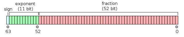
and represents a real number $x \in \mathbb{R}$ with $sign$ , $e$ , and $b_i \in \{0,1\}$ such that

(-1)^{sign} (1.b_{51}b_{50}...b_{0})_2 \ 2^{e-1023}

or, potentially more readable,

(-1)^{sign} \left ( 1 + \sum_{i=1}^{52} b_{52-i} 2^{-i} \right ) \times 2^{e-1023}.

In essence, floating point numbers have three main components: the sign, the exponent (which gives us scale), and the fraction (which gives us precision). This is much like scientific notation, e.g., $5.916829373 \times 10^{23}$ , but in base two. For the following example, we’ll use base ten scientific notation, since it’s a bit easier to work with.

This format allows for two numbers to be multiplied and divided without loss of precision:

\begin{align} & (5.916829373 \times 10^{23}) \times (7.208209342 \times 10^{-51}) \\[2.5ex] = & 5.916829373 \times 10^{23} \times 7.208209342 \times 10^{-51} \\[2.5ex] = & 5.916829373 \times 7.208209342 \times 10^{23} \times 10^{-51} \\[2.5ex] = & (5.916829373 \times 7.208209342) \times (10^{23} \times 10^{-51}). \end{align}

This works great for multiplication and division (due to associativity and commutativity) as we can rearrange and compute these operations separately. This is not the case, however, for addition and subtraction:

\begin{align} & (5.916829373 \times 10^{23}) + (7.208209342 \times 10^{-51}) \\[2.5ex] != & (5.916829373 \times 7.208209341) + (10^{23} \times 10^{-51}) \end{align}

and so we end up with having to round off. In fact, in this case, we lose the fact that we added anything at all!

\begin{align} & (5.916829373 \times 10^{23}) + (7.208209342 \times 10^{-51}) \\[2.5ex] = & (5.916829373 \times 10^{23}). \end{align}

This may seem obvious, but it means that the floating point numbers have gaps. For each floating point (except the largest one), there is a next one. More importantly, the gaps between each floating point number and the next one change as the floating point numbers get larger. We can see this in Python:

In [1]: import sys
In [2]: plus_epsilon_identity(x, eps):
            return x + eps == x
In [3]: eps = sys.float_info.min
In [4]: plus_epsilon_identity(0.0, eps)
Out[4]: False
In [5]: plus_epsilon_identity(1.0, eps)
Out[5]: True
In [6]: plus_epsilon_identity(1.0e20, 1.0)
Out[6]: True

Now, given x_0, if we choose h so small such that x_0 + h == x_0, then

\frac{f(x_0 +h) - f(x_0)}{h} = \frac{f(x_0) - f(x_0)}{h} = \frac{0}{h} = 0.

This is clearly undesirable. To take this on we first need to understand the size of the gaps. In Python:

In  [7]: def eps(x):
             e = float(max(sys.float_info.min, abs(x)))
             while not plus_epsilon_identity(x, e):
                 last = e
                 e = e / 2.
             return last
In [8]: eps(1.0)
Out[8]: 2.220446049250313e-16
In [9]: eps(1.0e10)
Out[9]: 1.1102230246251565e-06
In [10]: eps(1.0e20)
Out[10]: 11102.230246251565

It turns out that a good choice for h is¹

h = \sqrt{u} \times \max(\left \vert x \right \vert, 1)

where $u = eps(1)$ . We can update our finite difference method accordingly:

In [11]: def finite_difference(f, x, h=None):
             if not h:
                 h = sqrt(eps(1.0)) * max(abs(x), 1.0)
             return (f(x+h) - f(x))/h

We can test this out on some functions which we know the derivative of:

In [12]: def error(f, df, x):
             return abs(finite_difference(f, x) - df(x))

In [13]: def error_rate(f, df, x):
            return error(f, df, x) / df(x)

In [14]: f, df = lambda x:x**2, lambda x:2*x
In [15]: error_rate(f, df, 1.0)
Out[15]: 7.450580596923828e-09
In [16]: error_rate(f, df, 1.0e5)
Out[16]: 9.045761108398438e-09
In [17]: error_rate(f, df, 1.0e20)
Out[17]: 4.5369065472e-09

In [18]: import math
In [19]: f, df = math.sin, math.cos
In [20]: error_rate(f, df, 1.0)
Out[20]: 1.2780011808656197e-08
In [21]: error_rate(f, df, 1.0e10)
Out[21]: 1.002014830004253
In [22]: error_rate(f, df, 1.0e20)
Out[22]: 0.9999999999998509

At this point we have essentially minimized the total error, both from the finite difference method and from computational round off.² As such, it would be easy to think this is as good as it gets. Surprisingly, though, with the help of the complex numbers, we can take this even further.

Complex analysis

Have you ever tried to solve $x^2 + 1 = 0$ ? If you have, you’ll know that it is impossible for all $x \in \mathbb{R}$ . We would need $x^2 = -1$ , but when we square a real number, it will stay positive if it’s positive, become positive if it’s negative, or stay $0$ if it’s $0$ . In order to solve this, we actually need to bring in a whole new set of numbers: the imaginary numbers. We define

i = \sqrt{-1}

and then, together with the real numbers, build the complex numbers as:

\mathbb{C} = \{x + iy \ \forall \ x,y \in \mathbb{R}^2 \}.

We can now solve our dreaded $x^2 + 1 = 0$ with $\pm i$ . In fact, all polynomials of degree $n$ will have $n$ zeros in $\mathbb{C}$ . There is plenty to explore in the realm of complex analysis, but we are going to focus on the derivative.

Example 3

Consider

f(x) = z^2.

Let $z = x + iy$ . Then

\begin{align} f(z) = f(x+iy) & = (x+iy)^2 = x^2 +2ixy + i^2y^2 \\[2.5ex] & = x^2 + 2ixy - y^2. \end{align}

Functions can always be written in terms of their real and imaginary parts, e.g., $f(x+iy) = u(x,y) + iv(x,y)$ . These can also be written as $\mathfrak{R}(f)$ and $\mathfrak{I}(f)$ , respectively. Note that both $u$ and $v$ are real valued functions, and $x$ and $y$ are both real numbers. In our example, we have

u(x,y) = x^2 - y^2 \ \mathrm{and} \ v(x,y) = 2xy.

We now have two equations, both of two variables, and so we can take four derivatives:

\begin{align} \frac{\partial u}{\partial x} = 2x & \frac{\partial v}{\partial x} = 2y \\[2.5ex] \frac{\partial u}{\partial y} = -2y & \frac{\partial v}{\partial y} = 2x. \end{align}

Note that:

\begin{align} \frac{\partial u}{\partial x} = \frac{\partial v}{\partial y}, & \frac{\partial u}{\partial y} = -\frac{\partial v}{\partial x}. \end{align}

These are the Cauchy-Riemann equations and they hold for all analytic functions on $\mathbb{C}$ ! (See Marsden and Hoffman for a proof.) This theorem is going to give us the power to hack the derivative.

Hack the derivative

Given our function $f: \mathbb{C} \to X \subseteq \mathbb{C}$ , with the added restriction that $f: \mathbb{R} \to X \subseteq \mathbb{R}$ , we can rewrite as

f(z) = f(x+iy) = u(x,y) + iv(x,y)

Now, for $z \in \mathbb{C}$ we are only concerned with the subset of $\bar{z} \in \mathbb{R}$ . This tells us that for $\bar{z} = x + iy$ , we know that $y = 0$ . Plugging this in

f(\bar{z}) = f(x + i0) = u(x,0) + iv(x,0).

Similarly, we know that $f: \mathbb{R} \to X \subseteq \mathbb{R}$ , $f(\bar{z}) \in \mathbb{R}$ , which tells us that

v(x,0) = 0

and so

f(x,0) = u(x,0).

We’ve done a bit of algebra here, but all we are really saying is that $f$ returns real values for real valued input. We are going to use this and the Cauchy Riemann equations to our advantage.

We are attempting to estimate $\frac{df}{\partial x}$ . Since for all $\bar{z} \in \mathbb{R}$ we know $f=u$ ,

\frac{df}{\partial x} = \frac{\partial u}{\partial x} = \frac{\partial v}{\partial y}.

Using the definition of the derivative,

\frac{\partial v}{\partial y} = \lim_{h \to 0} \frac{v(x,y+h) - v(x,y)}{h}.

We know $\bar{z} \in \mathbb{R}$ , so we can substitute $y = 0$ and $v(x, 0) = 0$ :

\begin{align} \frac{\partial v}{\partial y} = & \lim_{h \to 0} \frac{v(x,h) - v(x,0)}{h} \\[2.5ex] = & \lim_{h \to 0} \frac{v(x,h)}{h}. \end{align}

eliminating both addition/subtraction operations that are so susceptible to rounding errors!

\frac{\partial v}{\partial y} = \lim_{h \to 0} \frac{v(x,h)}{h}.

Now, to estimate $\frac{df}{\partial x} = \frac{\partial v}{\partial y}$ , we again use a very small $h$

\frac{df}{\partial x} \approx \frac{v(x,h)}{h} = \frac{\mathfrak{I}(f(x+ih))}{h}.

This time, however, we will be able to use a much smaller $h$ . $\Box$

Python has native support for complex numbers, so we can implement this as

In [1]: import sys
In [2]: def complex_step_finite_diff(f, x):
           h = sys.float_info.min
           return (f(x+h*1.0j)).imag / h
In [3]: f, df = lambda x:x**2, lambda x:2*x
In [4]: complex_step_finite_diff(f, 1.0)
Out[4]: 2.0
In [5]: complex_step_finite_diff(f, 1.0e10)
Out[5]: 20000000000.0
In [6]: complex_step_finite_diff(f, 1.0e20)
Out[6]: 2e+20

The results here are stunning. We can formally test this out the same way as above:

In [7]: def cerror(f, df, x):
           return abs(complex_step_finite_diff(f, x) - df(x))

In [8]: def cerror_rate(f, df, x):
           return cerror(f, df, x) / x
In [9]: cerror_rate(f, df, 1.0)
Out[9]: 0.0
In [10]: cerror_rate(f, df, 1.0e10)
Out[10]: 0.0
In [11]: cerror_rate(f, df, 1.0e20)
Out[11]: 0.0

In [12]: import cmath

In [13]: f, df = cmath.sin, cmath.cos
In [14]: cerror_rate(f, df, 1.0)
Out[14]: 0.0
In [15]: cerror_rate(f, df, 1.0e10)
Out[15]: 0.0
In [16]: cerror_rate(f, df, 1.0e20)
Out[16]: 0.0

Again, stunning, but we can find some cases where it’s not perfect:

In [17]: cerror_rate(f, df, 1.0e5)
Out[17]: .110933124815182e-16
In [18]: f = lambda x: cmath.exp(x) / cmath.sqrt(x)
In [19]: df = lambda x: (cmath.exp(x)* (2*x - 1))/(2*x**(1.5))
In [20]: cerror_rate(f, df, 1.0)
Out[20]: 0.0
In [21]: cerror_rate(f, df, 1.0e2)
Out[21]: 1.1570932160552342e-16
In [22]: cerror_rate(f, df, 5.67)
Out[22]: 1.2795419601231268e-16
In [23]: cerror_rate(f, df, 1.0e3)
Out [23]: OverflowError: math range error

As you can see, the implementation of some complex functions have limitations. We also will not be able to use abs (its imaginary part is $0$ by definition) or a function with $<$ or $>$ in it (the complex numbers are not ordered).

The hack in the details

This is not an unknown method: the ACM Transactions on Mathematical Software published an article on the subject, The complex-step derivative approximation by Martins, Sturdza, and Alonso, in 2003. It also is not the only alternative to finite differencing. In fact, SIAM (the Society for Industrial and Applied Mathematics) issued a volume, Computational Differentiation: Techniques, Applications, and Tools (Siam Proceedings in Applied Mathematics Series ; Vol. 89), on the topic. We’ve only managed to scratch the surface here, and I make no claims of this being the optimal solution. (The optimal solution is almost entirely contextual, anyway.) There is plenty of the computational differentiation rabbit hole to left to explore.

The advantage of this method over finite differencing is quite stark (within the bounds where it works). Not only is it more accurate, but it also doesn’t involve the extra search for the right step size. Exploring these advantages and comparing them not only to finite differencing but all the other known methods is beyond the scope of an article such as this. But there is something quite interesting happening in the details here that offers a bit of insight into numerical computation. The “hack” that makes this work lies in the fact that $f(x,0) = u(x,0)$ and the substitution using the Cauchy-Riemann equations. But in general, $f(x,0) = u(x,0)$ is basically just the identity function. Yet somehow this gives us startlingly more accurate results.

The devil is in the details. The problems with the finite-differencing methods arise from the fact that basic mathematical truths, such as $x + \epsilon \ne x$ whenever $\epsilon \ne 0$ , do not hold true in floating point arithmetic. It is not actually that surprising that this is the case. Take the number $\pi$ , for example. Even with every atom in the visible universe acting as a bit in some hypothetical “universe computer”, you would not be able to represent the whole thing. It goes on forever. And there are uncountably more digits that are just the same way. In a lot of respects, it’s quite amazing how accurate many calculations can be made with floating numbers, like orbital mechanics and heat equations. It is important to remember that numerical computation is not abstract mathematics, and to have an awareness of what is happening under the hood. This hack gives us a fun way to take a peek, see where things break down, and use some other mathematics to patch it up.

From lecture notes posted by Karen Kopecky. ↩
It’s important to note that it’s a bit unreasonable to try and calculate a periodic function (let alone the derivative) at a floating point number where the gaps are far bigger than the periodicity. ↩