How to trick a neural network into thinking a panda is a vulture

Neural networks are magical

When I go to Google Photos and search my photos for ‘skyline’, it finds me this picture of the New York skyline I took in August, without me having labelled it!

When I search for ‘cathedral’, Google’s neural networks find me pictures of cathedrals & churches I’ve seen. It seems magical.

But of course, neural networks aren’t magic–nothing is! I recently read a paper, “Explaining and Harnessing Adversarial Examples”, that helped demystify neural networks a little for me.

The paper explains how to force a neural network to make really egregious mistakes. It does this by exploiting the fact that the network is simpler (more linear!) than you might expect. We’re going to approximate the network with a linear function!

It’s important to understand that this doesn’t explain all (or even most) kinds of mistakes neural networks make. There are a lot of possible mistakes! But it does give us some insight into one specific kind of mistake, which is awesome.

Before reading the paper, I knew three things about neural networks:

• they can perform really well on image classification tasks (so I can search for “baby” and find that adorable picture of my friend’s baby)
• everyone talks about “deep” neural networks on the internet
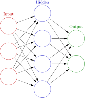
• they’re composed of layers of simple (often sigmoid) functions, which are often illustrated like this¹:
  

Mistakes

The fourth and final thing I knew about neural networks was: sometimes they make REALLY RIDICULOUS mistakes. Spoilers from later in this post: these are a couple of images, and how the neural network classifies them. We can convince it that a black image is a paper towel, and that a panda is a vulture!

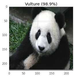
Now, none is this is too surprising to me–machine learning is my job, and machine learning habitually produces super weird stuff. But if we’re going to fix the super weird errors, we need to understand why they happen! We’re going to learn a little about neural networks, and then I’ll teach you how to trick a neural network into thinking a panda is a vulture.

Making our first prediction

We’re going to load a neural network, make some predictions, and then break those predictions. It’s going to be awesome. But first I needed to actually get a neural network on my computer.

I installed Caffe, which is neural network software written by some people at the Berkeley Vision and Learning Center at Berkeley. I picked it because it was the first one I could figure out, and that I could download a pre-trained network for. You could also try Theano or Tensorflow. Caffe has pretty clear installation instructions, which means it only took 6 hours of cursing before I got it to work.

If you want to install Caffe, I wrote up a procedure that will take you less than 6 hours. Just go to the neural-networks-are-weird repo and follow the instructions. Warning: it downloads approximately 1.5GB of data and needs to compile a bunch of stuff. These are the instructions to build it (3 lines!), which you can also find in the repository’s README:

git clone https://github.com/jvns/neural-nets-are-weird
cd neural-nets-are-weird
docker build -t neural-nets-fun:caffe .
docker run -i -p 9990:8888 -v $PWD:/neural-nets -t neural-nets-fun:caffe /bin/bash -c 'export PYTHONPATH=/opt/caffe/python && cd /neural-nets && ipython notebook --no-browser --ip 0.0.0.0'

This starts up an IPython notebook server on your computer where you can start making neural network predictions in Python. It should be running on port 9990 on localhost. If you don’t want to play along, that’s also totally fine. I included pictures in this article, too!

Once we have the IPython notebook up and running, we can start running code and making predictions! From here on I’m just going to post pretty pictures and small code snippets, but the full code and the gnarly details are in this notebook.

We’re going to use a neural network called GoogLeNet², which won the ILSVRC 2014 competition in several categories. The correct classification was in the network’s top 5 guesses 94% of the time. It’s the network that the paper I read uses. (If you want a cool read, you can see how a human can’t do much better than GoogLeNet. Neural networks really are pretty magical.)

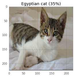
First off, let’s classify an adorable kitten³ using our network:

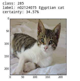
Here’s the code to classify the kitten.

image = '/tmp/kitten.png'
# preprocess the kitten and resize it to 224x224 pixels
net.blobs['data'].data[...] = transformer.preprocess('data', caffe.io.load_image(image))
# make a prediction from the kitten pixels
out = net.forward()
# extract the most likely prediction
print("Predicted class is #{}.".format(out['prob'][0].argmax()))

That’s all! It’s just 3 lines of code. I also classified a cute dog!

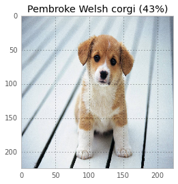
It turns out that this dog is not a corgi, but the colors are very similar. This network already knows dogs better than I do.

What a mistake looks like (featuring the queen)

The most amusing thing that happened while doing this work is that I found out what the neural network thinks the queen of England is wearing on her head.

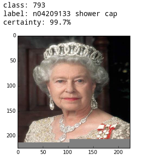
So now we’ve seen the network do a correct thing, and we’ve seen it make an adorable mistake by accident (the queen is wearing a shower cap ❤). Now… let’s force it to make mistakes on purpose, and get inside its soul.

Making mistakes on purpose

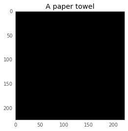
We’re going to need to do some math before we truly understand how this works, but first let’s look at some pictures of a black screen.

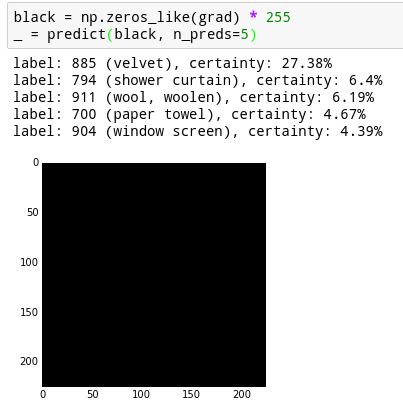
This completely black image is classified with probability 27% as velvet, and 4% as a paper towel. There are some other probabilities I haven’t displayed, and they add up to 100%.

I would like to figure out how to make the neural network more confident that this is a paper towel.

To do that, we need to calculate the gradient of the neural network. This is the derivative of the neural network. You can think of this as a direction to take to make the image look more like a paper towel.

To calculate the gradient, we first need to pick an intended outcome to move towards, and set the output probability list to be 0 everywhere, and 1 for paper towel. Backpropagation is an algorithm for calculating the gradient. I originally thought it was totally mystical, but it turns out it’s just an algorithm implementing the chain rule. If you want to know more, this article has a fantastic explanation of backpropagation.

Here’s the code I wrote to do that–it’s actually really simple to do! Backpropagation is one of the most basic neural network operations so it’s easily available in the library.

def compute_gradient(image, intended_outcome):
    # Put the image into the network and make the prediction
    predict(image)
    # Get an empty set of probabilities
    probs = np.zeros_like(net.blobs['prob'].data)
    # Set the probability for our intended outcome to 1
    probs[0][intended_outcome] = 1
    # Do backpropagation to calculate the gradient for that outcome
    # and the image we put in
    gradient = net.backward(prob=probs)
    return gradient['data'].copy()

This basically tells us what kind of shape the neural network is looking for at that point. Since everything we’re working with can be represented as an image, here it is–the output of compute_gradient(black, paper_towel_label), scaled up to be visible.

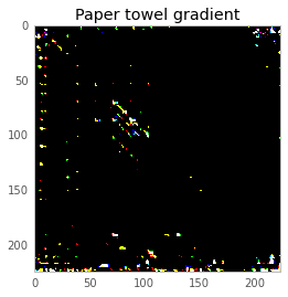
Now, we can either add or subtract a very light version of that from our black screen, and make the neural net think our image is either more or less like a paper towel. Since the image we’re adding is so light (the pixel values are less than 1/256), the difference is totally invisible. Here’s the result:

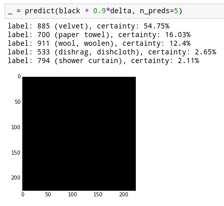
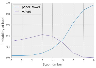
Now the neural network thinks our black screen is a paper towel with 16% certainty, instead of 4%! That’s really neat. But, we can do better. Instead of taking one step in the direction of a paper towel, we can take ten tiny steps and become a little more like a paper towel every step. You can see the probabilities evolve over time here. You’ll notice the probabilities are different than before because our step sizes are different (0.1 instead of 0.9).

and the final result:

And here are the pixel values that make up that image! They all started out at exactly 0, and you can see that we’ve mutated them to trick the network into thinking the image is a paper towel.

We can also multiply the image by 50 to get a better sense of what it looks like.

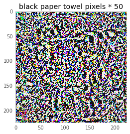
It doesn’t look like a paper towel to me, but maybe it does to you! I like to imagine all the swirls in that image are tricking the neural network into thinking it’s a paper towel roll. So, that’s the basic proof of concept, and some of the math. We’re going to go more into the math in a second, but first we’re going to have fun.

Having fun tricking the neural network

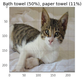
Once I figured out to do this, it was SO FUN. We can change a cat into a bath towel:

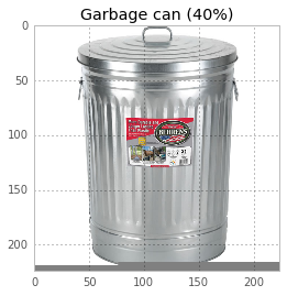
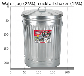
a garbage can into a water jug / cocktail shaker:

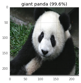
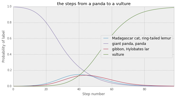
and a panda into a vulture. What better way to spend a Sunday morning?

This image showing how the probabilities progress from panda to vulture over 100 steps is pretty rad:

You can see the code to make all this work in the IPython notebook. It’s so fun.

Now, it’s time for a little more math.

How it works: logistic regression

First, let’s talk about the simplest way to classify an image–with logistic regression. What’s logistic regression? I’ll try to explain.

Suppose you have a linear function, for classifying whether an image was a raccoon or not. How would we use that linear function? Well, suppose your image had only 5 pixels in it. $(x_1, x_2, x_3, x_4, x_5)$, between 0 and 255. Our linear function would have weights, for instance $(23,-3,9,2,-5)$, and then to classify an image, we’d take the inner product of the pixels and the weights:

Now, suppose the result is 794. Does 794 mean it’s a raccoon or it’s not? Is 794 a probability? 794 IS NOT A PROBABILITY. A probability is a number between 0 and 1. Our result is a number between $-\infty$ and $\infty$. The way people normally get from a number between $-\infty$ to $\infty$ to a probability is by using a function called the logistic function: $S(t) = \frac{1}{1 + e^{-t}}$

which looks like this:

S(794) is basically 1, so if we got 794 out of our raccoon weights, we’d determine that it’s 100% a raccoon. This model–where we first transform our data with a linear function and then apply the logistic function to get a probability–is called logistic regression, and it’s a super simple and popular machine learning technique.

The “learning” part of machine learning is how to determine the right weights (like $(23,-3,9,2,-5)$) given a training dataset so that our probabilities can be as good as possible. The bigger the training set, the better!

Now that we understand what logistic regression is, let’s talk about how to break it!

Breaking logistic regression

There’s a gorgeous blog post called Breaking Linear Classifiers on ImageNet by Andrej Karpathy, which explains how to break a simple linear model beautifully (it’s not quite a logistic regression, but it is a linear model). We’re going to use the same principles later to break neural networks.

Here’s an example (from Karpathy’s article) of some linear classifiers for various foods, flowers, and animals, visualized as images. (click to make it bigger)

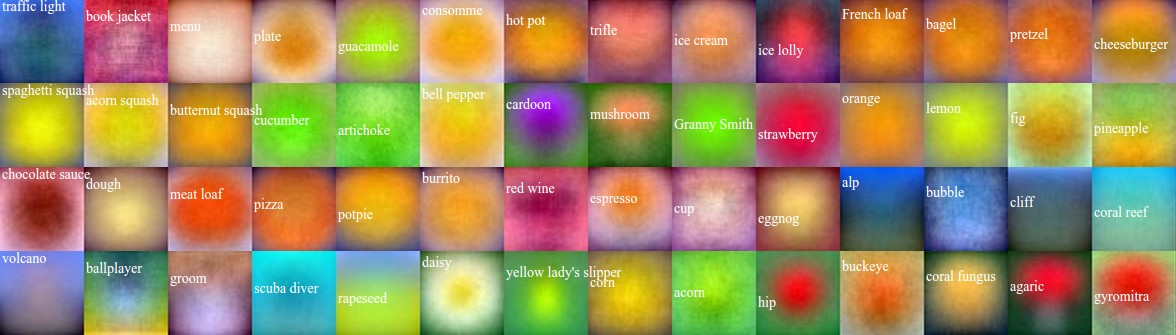
You can see that the “Granny Smith” classifier is basically asking “is it green?” (not the worst way to find out!) and the “menu” one has discovered that menus are often white. Karpathy explains this super clearly:

For example, Granny Smith apples are green, so the linear classifier has positive weights in the green color channel and negative weights in blue and red channels, across all spatial positions. It is hence effectively counting the amount of green stuff in the middle.

So, if I wanted to trick the Granny Smith classifier into thinking I was an apple, all I’d have to do is

• figure out which pixels it cares about being green the most
• tint those green
• profit!

So now we know how to trick a linear classifier. But a neural network isn’t linear at all–it’s highly nonlinear! Why is this even relevant?!

How it works: neural networks

I’m going to be totally honest here: I’m not a neural networks expert, and my neural networks explanations are not going to be great. Michael Nielsen has written a book called Neural Networks and Deep Learning which is very well-written. I’m also told that Christopher Olah’s blog is quite good.

What I do know about neural networks is: they’re functions. You put in an image, and you get out a list of probabilities, one for each class. Those are the numbers you’ve been seeing next to the images throughout this article. (is it a dog? nope. A shower cap? nope. A solar dish? YES!!)

So a neural network is, like, 1000 functions (one for each probability). But 1000 functions are really complicated to reason about. So what neural networks people do is, they combine the 1000 probabilities into a single “score”. They call this the “loss function”.

This loss function for each image depends on the actual correct output for the image. So suppose that I have a picture of an ostrich, and the neural network has output probabilities $p_j$ for $j = 1 \ldots 1000$, but the probabilities I WANT for the ostrich are $y_j$. Then the loss function is

And let’s say the label corresponding to ‘ostrich’ is number 700. Then $y_{700} = 1$, all the rest of the $y_j$ are 0, and $L = - \log p_{700}$.

The important thing here is to understand is that a neural network gives you a function from an image (the panda) to a final value of the loss function (a number, like 2). Because it’s a single-valued function, taking the derivative (or gradient) of that function gives you another image. You can then use that image to trick the neural network, using what we’ve talked about in this article!

Breaking neural networks

Here’s how all our words about breaking a linear function / logistic regression relate to neural networks! This is the math you’ve been waiting for! Near our image (an adorable panda), the loss function looks like

where the gradient grad is $\nabla L(x)$. This is because of calculus. In order to change the loss function by a lot, we want to maximize the dot product of the direction we’re moving delta and the gradient grad. Let’s calculate grad via our compute_gradient() function, and draw it as a picture:

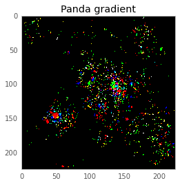
The intuition behind what we want to do is–we want to create a delta which emphasizes the pixels in the picture that the neural network thinks are important. Now, let’s suppose grad was $(-0.01, -0.01, 0.01, 0.02, 0.03)$.

We could make $\text{grad} \cdot \text{delta}$ big by taking $\text{delta} = (-1, -1, 1, 1, 1)$, to get 0.08. Let’s try that! In code, that’ll be delta = np.sign(grad). And when we move it by that amount, sure enough – now the panda’s a weasel.

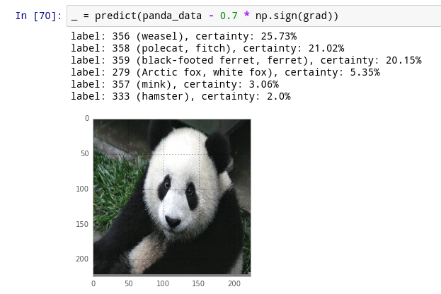
But, why? Let’s think about the loss function. We started out by looking at the probability it was a panda, which was 99.57%. $-\log(0.9957) = 0.0018$. Pretty small! So adding a multiple of delta should increase our loss function (and make it less like a panda), and subtracting a multiple of delta should decrease our loss function (and make it more like a panda). But actually the opposite happens! I’m still confused about this.

The dog you can’t trick

Now that we know the math, a short story. I also tried to trick the network about this adorable dog from before:

But the dog was highly resistant to being classified as something other than a dog! I spent some time trying to convince it that the dog was a tennis ball but it remained, well, a dog. Other kinds of dogs! But still a dog.

I ran into Jeff Dean (who works on neural nets at Google) at a conference, and asked him about this. He told me that there are a ton of dogs in the training set for this network, way more than there are pandas. So he hypothesized that the network is better-trained to recognize dogs. Seems plausible!

I think this is pretty cool and it makes me feel more hopeful about training networks that are more accurate.

One other funny thing about this conversation–when I tried to trick the network into thinking a panda is a vulture, it spent a while thinking it was an ostrich in the middle. And when I asked Jeff Dean this question about the panda and the dog, he mentioned off-hand “the panda ostrich space” without me bringing up ostriches at all! I thought it was cool that he’s clearly spent enough time with the data & these neural networks to just know offhand that ostriches and pandas are somehow close together.

Less magic

When I started doing this, I didn’t know almost anything about neural networks. Now that I’ve tricked them into thinking a panda is a vulture and seen how it’s smarter at dealing with dogs than pandas, I understand them a tiny bit better. I won’t say that I don’t think what Google is doing is magic any more–I’m still pretty confused by neural nets. There’s a lot to learn! But tricking them like this removes a little of the magic, and now I feel better about them.

And so can you! All the code to reproduce this is in this neural-networks-are-weird repo. It uses Docker so you can get it installed easily, and you don’t need a GPU or a fancy computer. I did all this on my 3-year-old GPU-less laptop.

And if you want to feel even better, read the original paper! (“Explaining and Harnessing Adversarial Examples”). It’s short, well written, and tells you more that I didn’t go into here, including how to use this trick to build better neural networks!

Thanks to Mathieu Guay-Paquet, Kamal Marhubi, and others for helping me with this article!